1 Introduction
1.1 Data
In geophysics, we measure many different types of data depending on the physical method being used.
1.1.1 Example Data
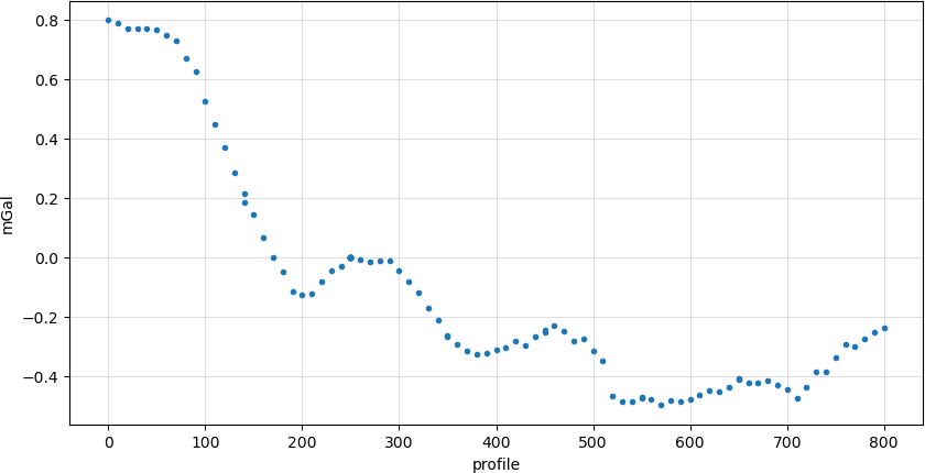
Data can be simple point-like measurements associated to measuring positions, like the Bouguer anomaly in gravity (measurement, reduced by temporal, global field and topographic effects).
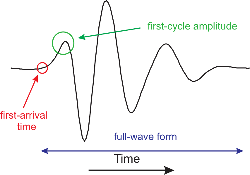
In seismology and seismics, wave trains (time series of acceleration, velocity or position) are acquired, of which either the whole series (full waveform), the first arrival, or an amplitude is used.
In travel-time tomography, an example that we extensively use here, the first arrivals, i.e. traveltimes between shots and geophones, are used.
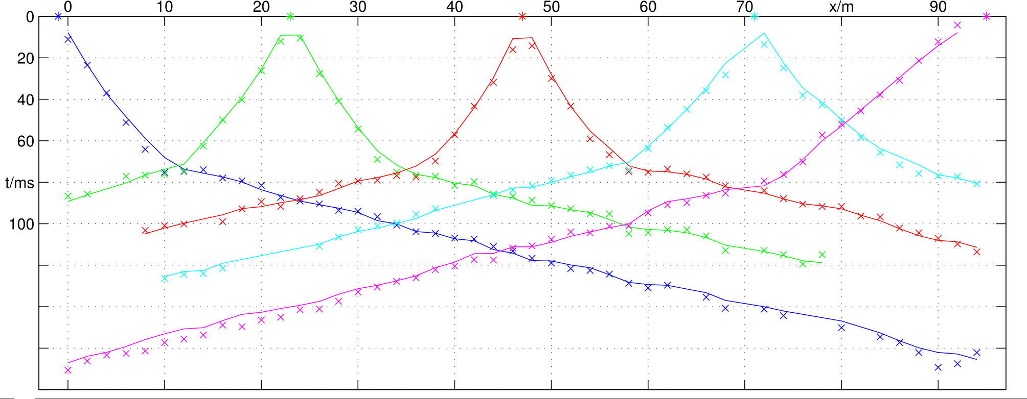
So they are associated to measuring points, but also depending on the experiment.
In electrical resistivity tomography (ERT), even more electrodes come into play, using different current and voltage combinations.
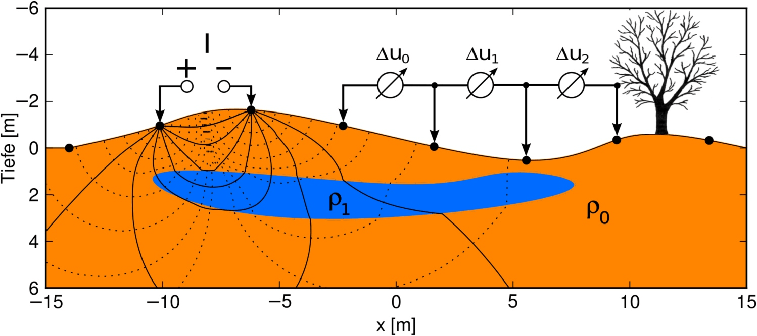
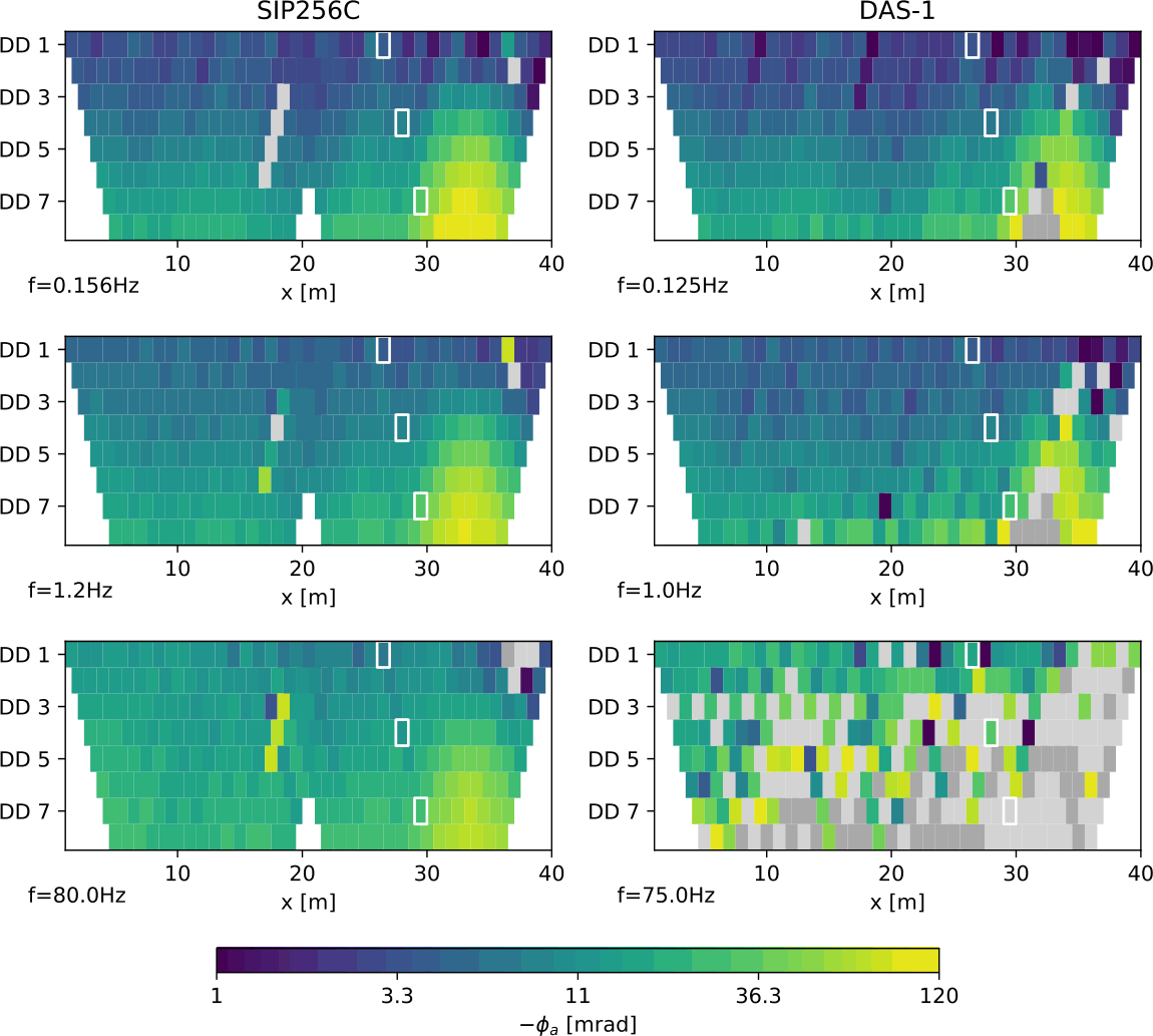
As a result, we obtain a pseudosection of apparent resistivity, which is however, even though organized in a logical/geometrical way, just a colored representation. These experiments can be repeated in time, opening the temporal dimension. In spectral IP (induced polarization), we even measure pseudosections for different frequencies, and introduce further dimensions.
1.1.2 Data organization
In geophysics, there are rules to look at data across several dimensions in space, time, or frequeny, but eventually, the data are single values that are even independent or correlating across these dimensions.
- can be a discretized function of space, time or frequency, and plotted as such (curves)
- can depend on several sensor (shot/geophone, ABMN) and visualized as several curves or a coloured matrix (crossplot, pseudosection)
Data are subsumed in the data vector \[\textbf{d}=[d_1, d_2, \ldots, d_N]^T\] consist of true model response \(\bf f(m)\) plus noise \(\bf n\): \(\bf d=f(m)+n\)
1.2 Geophysical Workflow
A workflow for geophysical data consist
- Experimental design & synthetic models
- Data acquisition
- Preprocessing (QC, filtering)
- Error estimation
- Subsurface parameterization (model)
- Inversion
- Fit of data with model response
- Evaluation & resolution analysis
- Postprocessing & visualization
- Interpretation
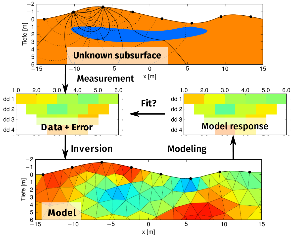
Here, we deal with the inversion, i.e. obtaining a subsurface model that fits the data. However, to this end, the previous steps (e.g., errors and model building) are important for carrying out inversion. Understanding the inversion process is crucial for the steps following inversion.
1.3 Model
is a numerical parameterization of subsurface and reflects our assumption of the truth by a simplification (reduction of complexity).
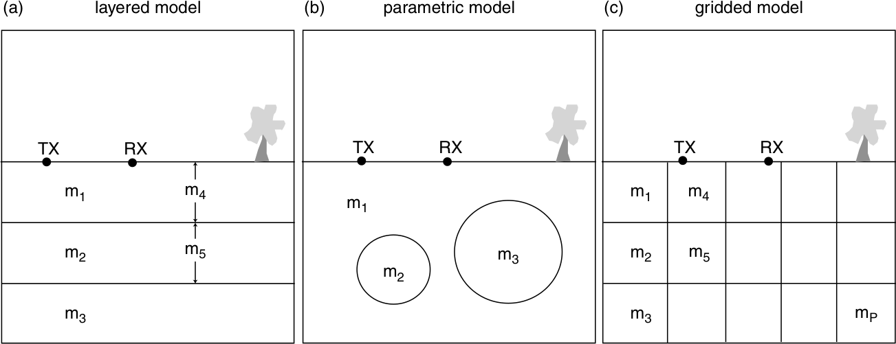
1.3.1 Model types
Models describe the distribution of one or more physical parameter in the subsurface, mostly by means of discrete values and possibly geometrical descriptions (layer thickness, anomaly size). There are some typical model types
Independent parameters:
- seismology: earthquake location, stress, principal axis
- gravity: position and depth of anomaly, size, density contrast
- spectroscopy (e.g. SIP): function parameters (e.g. Cole-Cole)
- layered model thicknesses and values (\(\rho\), \(v\))
Discrete functions of space, time, frequency
(same property aligned along axes)
- refraction: depth (and velocity) of refractor
- distribution of a parameter in space (and time)
- spectroscopy: Fourier or Debye distribution
- e.g. 2D/3D resistivity/velocity/density distribution
In all cases, the subsurface is described by model vector \(\textbf{m}=[m_1, m_2, \ldots, m_M]^T\), which can consist of physical or geometrical values.
1.4 Inversion
\[ \vb d \approx \vb f(\vb m) \]
\[ \vb d = \vb f(\vb m) \]
Because \(\vb d=\vb f(\vb m)+\vb n\) contains random noise \(\vb n\) that is not to be explained.
1.4.1 Minimization problem
\[ \Phi_d=\|{\vb d - f(m)}\|^2_2 = \sum_i^N (d_i-f_i(\vb m))^2 \rightarrow \min \]
Take into account errors: Explain model within error (\(\boldsymbol{\epsilon}\)) bounds \[ \Phi_d = \| \frac{\vb d-f(m)}{\boldsymbol{\epsilon}}\|^2_2 = \sum_i^N \left(\frac{d_i-f_i(\vb m)}{\epsilon_i}\right)^2 \| \rightarrow \min \]
error model \(\boldsymbol{\epsilon}=[\epsilon_1, \epsilon_2, \ldots, \epsilon_N]^T\) (assumption of noise standard deviation)
1.4.2 Correctness
In mathematics, we distinguish well and ill posed problems.
- There is a solution,
- it is uniquely defined &
- depends steadily from input data (small variations lead to small model deviations)
- There is no model to fit the data perfectly
- Many models can fit the data within errors
- Small data variations can lead to large model deviations
It turns out that in geophysics most problems are of the second type. To cope with the non-uniqueness of possible solutions, there is Occam’s razor, a fundamental rule:
Pluralitas non est ponenda sine neccesitate!
(William of Ockham, Scottish philosopher and theologian, 14th century)
Entities must not be multiplied beyond necessity.
Of two competing theories, the simpler explanation is to be preferred.
From all models fitting the data, choose the simplest!
Inversion is to a large degree about the methodology of defining this through wise parameterization and regularization of the model.
We will first consider linear problems and study the methodology, before we treat non-linear problems by using what we learned from linear ones.