1 Introduction
In Geophysics, we are measuring a lot of different fields and try to use this for getting insight into the subsurface by using our knowledge of the physics. Numeric solutions are key to understanding the nature of the physical equations and to predict measurements. In the inverse problem, the solution of the forward problem, i.e. to predict synthetic data from a given parameter distribution, is the most important task and therefore also for the data analysis in geophysics.
1.1 Literature
There are hardly any textbooks covering numerical simulation methods in geophysical applications. Mostly, they are focused on the specific modelling purpose like electrodynamics (Haber), seismic wave modelling (Igel) geodynamics (Morra). Numerical recipes have been around for Fortran and C/C++, but higher-level programming languages are easier to use in academics. Besides the proprietary Matlab, Python has become the most widespread programming language in academia and research, which is why we use this here.
- Morra (2018): Pythonic Geodynamics - Implementations for fast computing, frei verfügbar, Dive into Python programming
- Warnick: Numerical Methods for Engineering : An Introduction Using MATLAB® and Computational Electromagnetics Examples
- Igel (2007): Numerical modelling in geophysics, short course
- Logg et al. (2011): Automated Solution of Differential Equations by the Finite Element Method: Link
- Press (2007): Numerical recipes: the art of scientific computing
- Haber (2015): Computational methods geophysical electromagnetics
1.1.1 Online references
- pyGIMLi: Python Geophysical Inversion and Modelling Library - the general-purpose library that we will make use here
- Homepage of Oskar package - finite element package based upon pyGIMLi with brilliant tutorials and examples
- Geoscience.XYZ - geoscience instruction material including the SimPEG code
- Fenics handbook - a general-purpose FE library
- Theory of electromagnetics - background of EM
1.2 Differential operators
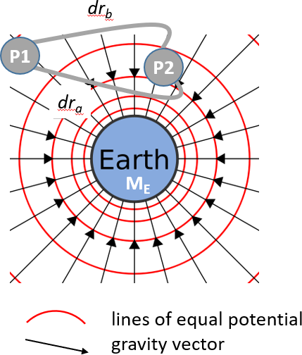
The physical fields are mostly governed by partial differential equations with differential operators in space and time. There are single derivatives in space \(\pdv{x}\) or time \(\pdv{t}\). All derivatives into all spatial dimensions are subsumed in the nabla operator \(\grad=(\pdv x, \pdv y, \pdv z)^T\). The (negative) gradient of a potential is the corresponding vector field with directions perpendicular to the isosurfaces into the direction of decreasing potential.
The divergence applies the nabla operator to a vectorial field by the dot product: \[\div \vb F = \pdv{F_x}{x} + \pdv{F_y}{y} + \pdv{F_z}{z}\] The divergence of a field describes the source strength using Gauss’ law.
Gauss’ law:
what’s in (volume) comes out (surface) \[\int_V \div\vb F\ dV = \iint_S \vb F \vdot \vb n\ dS\]

The curl (rotation) operator occurs particularly in electromagnetic problems, where magnetic fields are caused by (conduction or displacement) currents and electric fields infer changes in the magnetic field. It is described by the cross-product between nabla operator and the field \[\curl \vb F = (\pdv{F_z}{y}-\pdv{F_y}{z}, \pdv{F_x}{z}-\pdv{F_z}{x}, \pdv{F_y}{x}-\pdv{F_x}{y})^T\]
Stokes law:
what goes around comes around \[\int_S \curl \vb F \vdot \vb dS = \iint_S \vb F \vdot \vb dl\]

There are two laws concerning curl fields:
- curls have no divergence: \[\div (\curl \vb F)=0 \tag{1.1}\]
- potential fields have no curl \[\curl (\grad u)=0 \tag{1.2}\]
1.3 Partial differential equations (PDEs)
Mostly: solution of partial differential equations (PDEs) for either scalar (potentials) or vectorial (fields) quantities.
1.3.1 Types of partial differential equations
Let \(u\) denote the searched function, \(f\) the source (force) and \(a\)/\(c\) are material parameters. Depending on the occurring derivatives, we distinguish three main
- elliptic (potentials) PDE of Poisson type \[-\nabla^2 u=f\] or Helmholtz type \[\nabla^2 u + k^2 u = f\]
- parabolic (diffusion processes) PDE \[-\nabla^2 u + a \pdv{u}{t} \frac{\partial u}{\partial t}=f\]
- hyperbolic (wave propagation) PDE \[-\nabla^2 u + c^2 \frac{\partial^2 u}{\partial t^2}=f\], which can also have a diffusive term \[\frac{\partial^2\ u}{{\partial x}^2} - c^2\frac{\partial^2 u}{\partial t^2} = 0\]
There are also other types:
- coupled \(\nabla\cdot u=f\) & \(u = K \nabla p=0\) (Darcy flow)
- nonlinear \((\nabla u)^2=s^2\) (Eikonal equation)
1.3.2 Potential probleme - Poisson equation
A potential field \(u\) generates a vector field \(\vb F=-\nabla u\) along its gradient, which in turn can cause some flow \(\vb j=a \vb F\), where \(a\) is some sort of conductivity (electric, hydraulic, thermal). Part of the flow is generated (injected) by our source, denoted as \(\vb j_s\).
The continuity of flow states that the divergence of total current \(\vb j + \vb j_s\) vanishes, i.e., taking Gauss’ law into account, in an arbitrary volume the sum of the currents flowing into (its normal vector) is zero:
\[ -\div (a \nabla u) = \div \vb j_s \]
The operator on the left-hand side is called Laplace operator, a (negative) second derivative, i.e. the first derivative of the conductivity-weighted potential gradient. Discarding \(a\) for a moment, a increasing first derivative is a positive curvature, typically a minimum of a curve. Since we have a negative second derivative, we have a negative curvature, typically a maximum, at in the vicinity of a source (the right-hand side), where current flows into the system.
1.3.3 Diffusion problems
1.3.3.1 The heat equation in 1D
sought: Temperature \(T\) as a function of space and time
heat flux density \(\vb q = \lambda\grad T\)
\(q\) in W/m², \(\lambda\) - heat conductivity/diffusivity in W/(m.K)
Fourier’s law: \(\pdv{T}{t} - a \nabla^2 T = s\) (\(s\) - heat source)
temperature conduction \(a=\frac{\lambda}{\rho c}\) (\(\rho\) - density, \(c\) - heat capacity)
1.3.4 Flow and transport
1.3.4.1 Darcy’s law
volumetric flow rate \(Q\) caused by gradient of pressure \(p\)
\[ Q = \frac{k A}{\mu L} \Delta p \]
\[\vb q = -\frac{k}{\mu} \nabla p \]
\[\div\vb q = -\div (k/\mu \grad p) = 0\]

1.3.4.2 Stokes equation
\[ \mu \nabla^2 \vb v - \grad p + f = 0 \]
\[\div\vb v = 0 \]
1.3.5 Electromagnetics
1.3.5.1 Maxwell’s equations
- Faraday’s law: currents & varying electric fields \(\Rightarrow\) magnetic field \[ \curl \vb H = \pdv{\vb D}{t} + \vb j \]
- Ampere’s law: time-varying magnetic fields induce electric field \[ \curl\vb E = -\pdv{\vb B}{t}\]
- \(\div\vb D = \varrho\) (charge \(\Rightarrow\)), \(\div\vb B = 0\) (no magnetic charge)
- material laws \(\vb D = \epsilon \vb E\) and \(\vec B = \mu \vb H\)
1.3.6 Helmholtz equations
e.g. from Fourier assumption \(u=u_0 e^{\imath\omega t}\)
\[ \div (a\grad u) + k^2 u = f \]
- Poisson operator assembled in stiffness matrix \(\vb A\)
- additional terms with \(u_i\) \(\Rightarrow\) mass matrix \(\vb M\)
\[ \Rightarrow \vb A + \vb M = \vb b \]
\[ \nabla^2 u + k^2 u = f \]
results from wavenumber decomposition of diffusion or wave equations
approach: \(\vb F = \vb{F_0}e^{\imath\omega t} \quad\Rightarrow\quad \pdv{\vb F}{t}=\imath\omega\vb F \quad\Rightarrow\quad \pdv[2]{\vb F}{t}=-\omega^2\vb F\)
\[ \nabla^2 \vb F - a \nabla_t \vb F - c^2 \nabla^2_t \vb F = 0 \]
\[ \Rightarrow \nabla^2\vb F - a\imath\omega\vb F + c^2 \omega^2\vb F = 0 \]
1.3.7 Wave phenomena
1.3.7.1 Hyberbolic equations
Acoustic wave equation in 1D \[ \pdv[2]{u}{t} - c^2\pdv[2]{u}{x} = 0 \]
\(u\)..pressure/velocity/displacement, \(c\)..velocity
Damped (mixed parabolic-hyperbolic) wave equation \[ \pdv[2]{u}{t} - a\pdv{u}{t} - c^2\pdv[2]{u}{x} = 0 \]
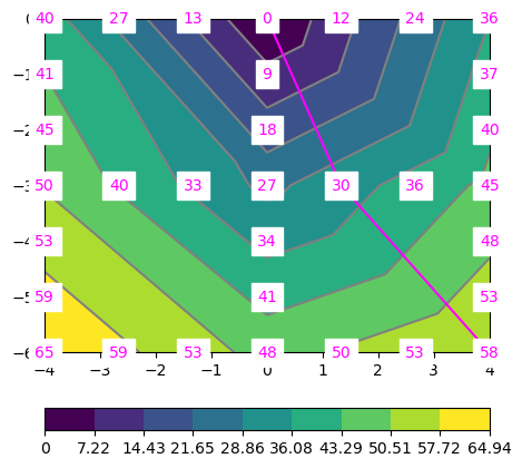
1.3.7.2 The eikonal equation
Describes first-arrival times \(t\) as a function of velocity (\(v\)) or slowness (\(s\))
\[ |\grad t| = s = 1/v \]
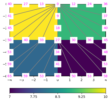
Finally, we have the traveltimes at all nodes, including the ray paths in the individual cells.
1.4 Content
We are going to introduce three main methods to solve PDEs after which the following chapters are organized:
- The Finite Difference (FD) method (FDM)
- The Finite Element (FE) method (FEM)
- The Finite Volume (FV) method (FVM)
We start solving the Poisson equation (elliptic PDE) in 1D, eventually using all three methods. For FD, there is just a quick look to how it is working in 2D and 3D and in FV none at all.
We dive into solving a parabolic equation, i.e. the instationary heat equation, first using FD, and later FE.
The main method to be used is FE, as it represents the most widely use and most flexible of these three. Here, we go, like in FD, from the Poisson equation to the instationary heat equation.
Next, we increase the spatial dimension to 2D, using irregularly structured triangle meshes. Unlike in 1D, it is tedious to program FE by ourselves. Therefore, we will use the Python package pyGIMLi for building meshes and setting up the matrices.
Using FE, we go from the 2D Poisson equation to the complex-valued Helmholtz equation as it is arising for problems transferred from the time domain into the frequency domain. The example being used here is 2D diffusion of plane-wave electromagnetic fields into the air, as used in the Magnetotelluric (MT) method.
Finally, it is shown how the vector electromagnetic diffusion problem is solved by using problem-adapted elements and boundary conditions, both in frequency and time domain. Finally, the performance of large-scale problems, is discussed.