3 Finite Elements

3.1 History and background

[1943] Courant: Variational Method
[1956] Turner, Clough, Martin, Topp: Stiffness
[1960] Clough: Finite Elements for static elasticity
[1970-80] extension to structural, thermic and fluid dynamics
[1990] computational improvements
now main method for almost all PDE types

In geophysics, solution of Poisson equation with FE became popular in the 1970s, but were very limited in the 1980s, before they experienced a revival in the 1990s. From the 2000s to now they became predominant for a wide range of different problems.

3.2 Variational formulation of Poisson equation

We start with the continuity (Poisson with conductivity) problem: \[ -\div a \grad u = f \]

The equation is multiplied with a test (weighting) function $w$ and integrated over the whole modelling domain $\Omega$, leading to weak form

\[ -\int_\Omega w \div a \grad u \dd\Omega = \int_\Omega w f \dd\Omega \]

Now we use the vector identity $ (bc) = bc + b c $

or, rewritten, $-b\div \vb c = \grad b \cdot \vb c - \div(b\vb c)$

with $b=w$ and $\vb c=\grad u$ to obtain

\[ \int_\Omega \grad w \vdot a \grad u \dd\Omega - \int_\Omega \div(w a \grad u) \dd\Omega = \int_\Omega w f \dd\Omega \]

We make use of Gauss’ law $\int_\Omega \div \vb A = \int_\Gamma \vb A \cdot \vb n$ to transform the second term into a surface integral, yielding

\[ \int_\Omega a \grad w \vdot \grad u \dd\Omega - \int_\Gamma a w \grad u \dd\Gamma = \int_\Omega fw \dd\Omega \]

Let our approximation $u_h$ be constructed by a number of shape functions $v_i$ with the coefficients $u_i$:

\[u_h(\vb r)=\sum_i u_i v_i(\vb r)\]

This shows an important feature of Finite Elements: it is a function in the whole modelling domain, constructed by basis . We can then satisfy the latter equation

\[ \sum_i \int_\Omega a \grad w \vdot \grad v_i \dd\Omega - \sum_i \int_\Gamma a w \grad v_i \dd\Gamma = \int_\Omega fw \dd\Omega \]

The Galerkin method now consists of the idea to choose the test functions out of the same space as the shape (trial) functions $w_i \in {v_i}$ so that for all $v_j$ holds

\[ \sum_i u_i \int_\Omega a \grad v_j \vdot \grad v_i \dd\Omega - u_i \int_\Gamma a v_j \grad v_i \dd\Gamma = \int_\Omega f v_j \dd\Omega \]

For every $j$, this represents an equation for the different coefficients $u_i$, where the integral is a predefined factor that can be put into a vector that is multiplied with the coefficient vector $\vb u={u_i}$. Written for all $j$, this represents a matrix-vector equation

\[ \vb A \vb u = \vb b \]

with the so-called stiffness matrix $\vb A$. Although generally all possible functions can be chosen for $v_i$, mostly we choose them in such a way that $\grad v_i$ is simple to compute and $\grad v_i \vdot \grad v_j$ is zero in most of the subsurface. To this end, we divide subsurface in sub-volumes $\Omega_c$ with constant $a_i$ and $\grad v_i$ being zero outside of the corresponding cell.

The functions $v_i$ form a so-called function space that spans the solution, whose coefficients only depend on the right-hand side and the given boundary conditions in the middle term.

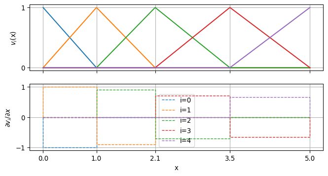
3.3 Hat functions

The simplest choice for the functions are piece-wise linear functions, so that the gradient is constant in every element. In order to achieve a continuous function and a sparse support, such a functions is associated to every node, where the value is 1 and decreases to 0 for the neighboring elements. In 1D these up-and-down functions are looking like a head. Every element is surrounded by two nodes “carrying” a hat.

import numpy as np
import matplotlib.pyplot as plt
x = np.array([0, 1., 2.1, 3.5, 5.0])
fig, ax = plt.subplots(figsize=(8, 4), nrows=2, sharex=True)
for i in range(len(x)):
    si = np.zeros_like(x)
    si[i] = 1
    ax[0].plot(x, si)
    dsdx = np.diff(si)/np.diff(x)
    ax[1].stairs(dsdx, x, ls="--", zorder=10, label=f"i={i}")

ax[0].set_xticks(x)
ax[0].set_yticks([0, 1])
ax[1].set_yticks([-1, 0, 1])
ax[0].grid()
ax[1].grid()
ax[1].legend()
ax[1].set_xlabel("x")
ax[0].set_ylabel(r"$v_i$(x)")
ax[1].set_ylabel(r"$\partial v_i/\partial x$");

The gradient of such a function is positive left of the node ($1/\Delta x_{i-1}$) and negative right of it ($-1/\Delta x_i$), and zero elsewhere. As it is piece-wise constant, the integrals are simple, to the right of the node $i$

\[ \int_\Omega a \grad v_i \vdot \grad v_{i+1} \dd\Omega = -\frac{a_i}{\Delta x_i^2} \cdot \Delta x_i = -\frac{a_i}{\Delta x_i} = C_i^{\text{right}}\]

and to the left \[ \int_\Omega a \grad v_i \vdot \grad v_{i-1} \dd\Omega = -\frac{a_{i-1}}{\Delta x_{i-1}^2} \cdot \Delta x_{i-1} = -\frac{a_{i-1}}{\Delta x_{i-1}} = C_i^{\text{left}}\]

The coefficients are called coupling coefficients as they couple the solution between nodes. For the same node $i$, the integral consists of two parts

\[ -\int_\Omega a \grad v_i \vdot \grad v_i \dd\Omega = \frac{a_{i-1}}{\Delta x_{i-1}^2}\Delta x_{i-1} + \frac{a_i}{\Delta x_i^2}\Delta x_i = \frac{a_{i-1}}{\Delta x_{i-1}} + \frac{a_i}{\Delta x_i} \]

For all other combinations of nodes (two or more nodes away), the coupling is zero.

\[ -\int_\Omega a \grad v_i \grad v_{i+2} \dd\Omega = 0 \]

This makes $\vb A$ a sparsely populated matrix, where only neighboring nodes have a matrix element, just like for Finite Differences. Note that for the latter the coupling coeffiecient was $a_i/\Delta x_i^2$, because the Finite Element method solves an integrated system, it has one power less.

Note

If the spacing $\Delta x$ is 1.0 everywhere, the FD system matrix equals the FE stiffness matrix and the solution is identical (for 1D). If $\Delta x$ is not 1.0 but constant, both sides of the equation are multiplied by it and the solution is still identical.

4 System (stiffness) matrix

Matrix integrating gradient of base functions for neighbors $A$ \[ \vb A_{i, i+1} = -\frac{a_i}{\Delta x_i^2} \cdot \Delta x_i \]

\[ A_{i,i} = \int_\Omega a \grad v_i \grad v_i \dd\Omega = -A_{i,i+1} + A_{i+1,i} \]

$\Rightarrow$ matrix-vector equation $\vb A \vb u = \vb b$ $\Rightarrow$

4.1 Boundary conditions

second term \[ - \int_\Gamma a v_i \grad v_j \dd\Gamma \]

4.2 Right-hand side vector

The right-hand-side vector $b=\int v_i f \dd\Omega$ also scales with $\Delta x$

e.g. $f=\div j_s$ $\Rightarrow$ $b=v_i j_s = _$

system identical to FD for $\Delta x=$const

Difference of FE to FD

Any source function $f(x)$ can be integrated on the whole space!

4.3 Solution

$\vb v$ holds the coefficient $u_i$ creating $u=\sum u_i v_i(x)$

Difference of FE to FD

$u$ is described on the whole space and approximates the solution, not the PDE!

Hat functions: $u_i$ potentials on nodes, $u$ piece-wise linear

Generality of FE

Arbitrary base functions $v_i$ can be used to describe $u$