4 Finite Volumes
4.1 Advection problems
Volume elements move with velocity \(\vb v\) and take (advectio=move with)
\[\pdv{T}{t} \Rightarrow \pdv{T}{t} + \dv{z}{t}\pdv{T}{z}\] in 3D \(\vb{v}\cdot\grad{T}\) \(\Rightarrow\) advection-dispersion equation
\[\pdv{T}{t} - \div a\grad{T} + \vb{v}\cdot\grad{T} = \div q_s\]
4.1.1 Continuity equation
\[ \dv{t}\int_V u(\vb r, t) \dd V = \int_V \pdv{u(\vb r, t)}{t} + \int_V \vb v \vdot \grad u(\vb r, t) \dd V \]
\[ \dv{t}\int_V u(\vb r, t) \dd V = \int_V \pdv{u(\vb r, t)}{t} + \int_{\partial V} u(\vb r, t) \vb v\vdot \vb n \]
Conservation of mass (\(u\)=\(\varrho\)) \(\Rightarrow\) divergence of flux \(u\vb v\)
\[ \pdv{u}{t} + \div(u \vb v) = 0 \]
can also be conservation of impuls or energy
4.1.2 Advection-dispersion equation (general)
\[ \pdv{u}{t}+\vb v\cdot\grad u - \div(a\grad u) = b u + f(\vb r, t)\]
flux \(\vb v\cdot\grad u\) (Advection), stiffness \(-\div(a\grad u)\) (Dispersion=Diffusion)
arising in Computational Fluid Dynamics
Solve, e.g., by pyGIMLi.solver.solveFiniteVolume (Link)
bc = dict(Dirichlet={4: 1.0, 3: 0.0}, Neumann={2: 1.0})
u = ps.solveFiniteVolume(mesh, a, b, f, bc=bc, t=times, c)
4.1.3 Computational magnetohydrodynamics
Magnetohydrodynamic induction equation
\[\pdv{\vb B}{t} = \curl \frac{1}{\mu\sigma} \curl \vb B + \curl(\vb v \cross \vb B)\]
Forces on fluid (induction, Coriolis, pressure, gravity, Lorentz) \[ \rho \pdv{\vb v}{t} + \rho (\vb v \cdot \grad) \vb v + \grad p = -2\omega\cross\vb v+\alpha T \vb g + \vb j \cross \vb B / \rho \]
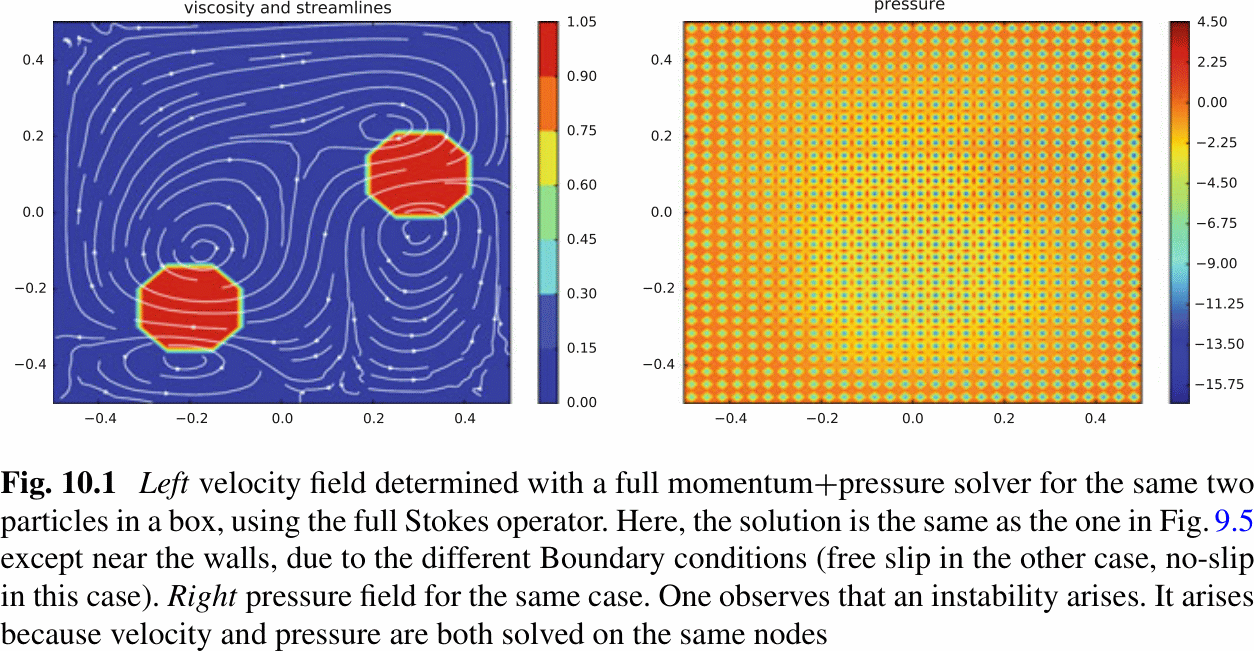
4.1.3.1 FE solution can bear instabilities
4.2 Finite Volume schemes
4.2.1 Simple 1D advection problem
\[\pdv{u}{t} + \pdv{v(u)}{x}=0\]
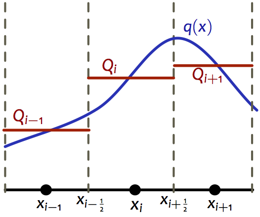
Solution \(u_i\) at node \(i\) represents average value over cell
\[ \overline{u}_i(t) = \frac{1}{x_{i+1/2}-x_{i-1/2}} \int_{x_{i-1/2}}^{x_{i+1/2}} u(x, t)\dd x \]
\[ \int_{t_1}^{t_2} \pdv{u}{t} = u(x, t_2)-u(x, t_1) = - \int_{t_1}^{t_2} \pdv{v(u)}{x} \]
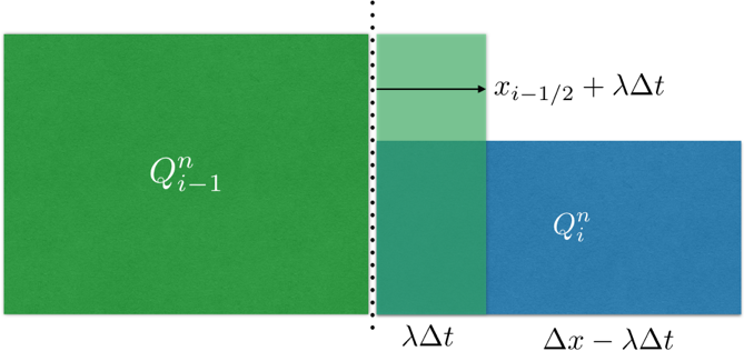
upwind method:
\[Q_i^{n+1} = Q_i^n - a\frac{\Delta t}{\Delta x} (Q_i^n-Q_{i-1}^N)\]
Lax-Wendroff (2nd order)
\[Q_i^{n+1} = Q_i^n - a\frac{\Delta t}{2\Delta x} (Q_{i+1}^n-Q_{i-1}^N)\]
\[+\frac12 (a\frac{\Delta t}{2\Delta x})^2 (Q_{i+1}^n-2Q_{i}^N+Q_{i-1}^N)\]
\[ u(x, t_2) = u(x, t_1) - \int_{t_1}^{t_2} \pdv{v(u)}{x} \]
\[ \overline{u}(t_2) = \frac{1}{x_{i+1/2}-x_{i-1/2}} \int_{x_{i-1/2}}^{x_{i+1/2}}\qty\Big(u(x,t_1) - \int_{t_1}^{t_2} \pdv{v(u)}{x}) \]
\[ \overline{u}(t_2) = \overline{u}(t_1) - \frac{1}{x_{i+1/2}-x_{i-1/2}} \qty\Big(\int_{t_1}^{t_2} v_{i+1/2} \dd t - \int_{t_1}^{t_2} v_{i-1/2} \dd t) \]
4.2.1.1 Result
\[ \pdv{\overline{u}_i}{t} +\frac{1}{\Delta x_i} (v_{i+1/2}-v_{i-1/2}) = 0 \]
Finite volume schemes are conservative as cell averages change through the edge fluxes. In other words, one cell’s loss is always another cell’s gain!
4.2.1.2 Visualization
4.2.2 Similarity to staggered (E, B) grid methods
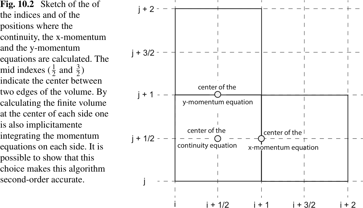
4.2.3 Conservation law (3D) problem
\[\pdv{\vb u}{t} + \div\vb v(u)= 0\]
volume integral over cell, using Gauss’ law
\[\int_{\Omega_i} \pdv{\vb u}{t}\dd\Omega+\int_{\Omega_i} \div\vb v(u) \dd\Omega = 0 = \int_{\Omega_i} \pdv{\vb u}{t}\dd\Omega+\int_{\Gamma_i} \vb v(u) \cdot \vb n \dd{\Gamma} \]
\[\Rightarrow \pdv{\overline{u}}{t} +\frac{1}{V_i}\int_{\Gamma_i}\vb v(u)\cdot \vb n \dd{\Gamma} =0 \]
4.2.4 Godunov’s scheme
- Define piece-wise constant approximation \(u^{n+1}\)
- Obtain solution for local Riemann problem at cell interfaces
- Average state variables from 2. over
4.3 The methods FD, FE and FV
approximates the partial derivatives by difference quotients (beware \(\Delta x\) and \(\Delta a\))
approximates the solution through base functions in integrative sense
approximates the solution by piecewise constant values and ensures conservation law by fluxes
4.3.1 Discontinuous Galerkin scheme
use Galerkin method (multiply test function and take as basis)
discretize fields by piece-wise constant functions
- fields are becoming discontinuous
communicate flux between elements by Riemann problem scheme
every element independent (also mesh size)
fully parallelized (element-wise)