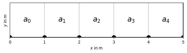
2 Finite Differences

Assume the general Poisson equation \[-\div(a\grad u)=f\]

with some conductivity \(a\), a source term \(f\) and the potential \(u\). This can be an electric potential with \(a=\sigma\), the hydraulic head with hydraulic conductivity \(k\), the temperature with the thermal conductivity \(\lambda\) or the gravity potential with \(a=1\). Note that we are using the form with the leading minus. First, \(-\grad u\) is typically the field (e.g. electric) and \(a\grad u\) is usually the flow (e.g. streaming velocity or current density) towards decreasing potential.

Neglecting \(a\) for a moment, the left-hand side is the second derivative, i.e. a curvature. A positive source field \(f\) leads to a negative curvature, i.e. a decreasing slope of the potential curve. This is a maximum of the potential caused by the source, e.g., an increased temperature for a heat source.

2.1 FD Approximation in 1D

The basic idea of the Finite Difference method is to approximate the partial derivatives by finite derivatives using a predefined discretization.

Approximate derivative operators by differences

\[ \pdv{u}{x}\approx\frac{\Delta u}{\Delta x} \]

The solution \(u\) is approximated by finite values \(u_i\) at points \(x_i\). Taking a Taylor expansion of any function f (describing the true solution) at a point \(x_0\) we obtain \[f(x)=f(x_0)+f'(x0)(x-x_0)+f''(x_0)(x-x_0)^2/2+\ldots\]

Mostly, the function is linearized, i.e. cut after the first derivative. The derivative is formulated from neighboring points \(x_j\). For describing the first derivative, one can use different differences:

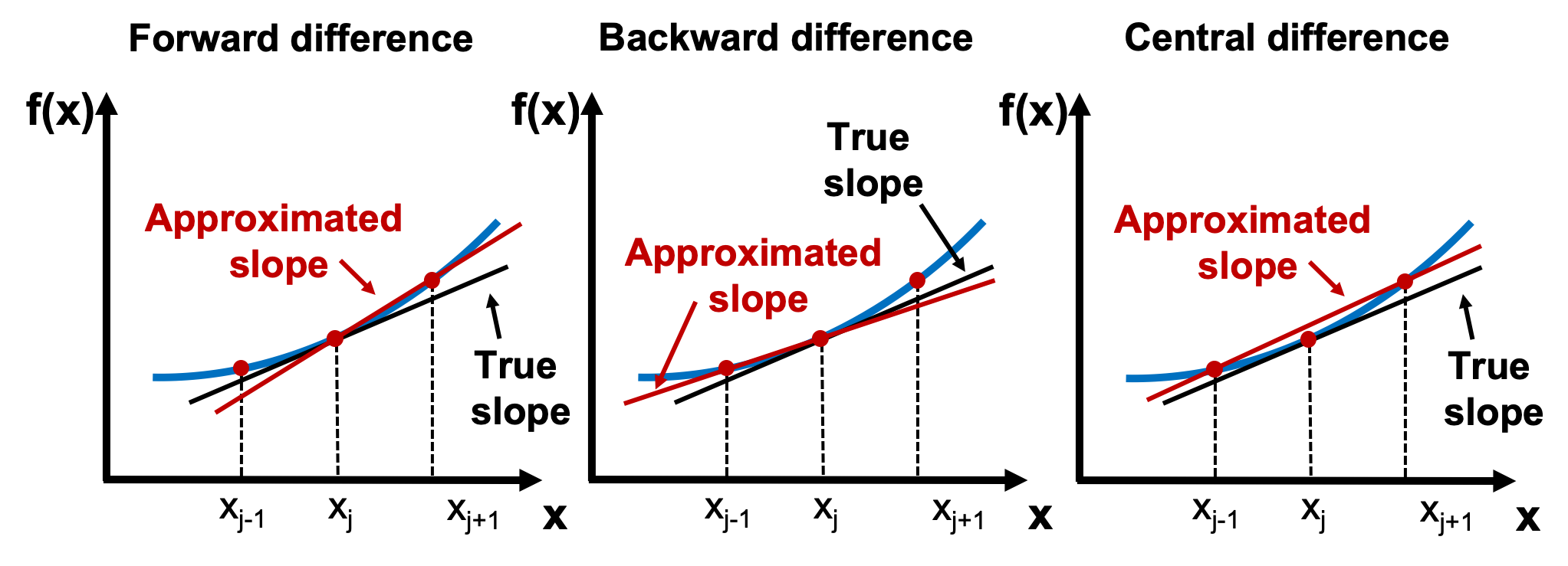
Forward, backward and central difference for 1D FD grid

For example, the difference of \(u\) between \(x_2\) and \(x_3\) is localized somehow between them \[ \dv*{u}{x}_{2.5} := (u_3-u_2) / (x_3-x_2) \]

For the Poisson equation, we need a second derivative, approximated by a central difference right and left of the point, e.g., for \(x_3\)

\[\pdv[2]{u_3}{x}\approx \frac{\dv*{u}{x}_{3.5}-\dv*{u}{x}_{2.5}}{(x_4-x_2)/2} = \frac{(u_4-u_3)/(x_4-x_3)-(u_3-u_2)/(x_3-x_2)}{(x_4-x_2)/2} \]

Hence, the second derivative is expressed by the value of a point and its neighbors, represented by a difference stencil.

2.1.1 Difference stencil

Assumption: equidistant discretization \(\Delta x\), conductivity 1

1st derivative: \([-1, +1] / dx\), 2nd derivative \([+1, -2, +1] / dx^2\)

Matrix-Vector product \(\vb{A}\cdot\vb{u}=\vb{f}\) with

\[ \vb{A} = \frac{1}{\Delta x} \begin{bmatrix} -1 & +2 & -1 & 0 & \ldots & & \\ 0 & -1 & +2 & -1 & 0 & \ldots & \\ \vdots & \vdots & \vdots & \ddots & \vdots & \\ \ldots & \ldots & 0 & -1 & +2 & -1 \end{bmatrix} \]

This is illustrated by the Finite Difference stencil (Figure 2.1): Every point, e.g. the red point, is constructed by using its neighbors.

Figure 2.1: 1D Finite-Difference stencil

2.1.2 FDM on the general Poisson equation

Assume the Poisson equation \[-\div(a\grad u)=f\] with a conductivity term \(a\), for a 1D discretization

\[ \pdv{(a \pdv*{u}{x})}{x} = a\pdv[2]{u}{x} + \pdv{a}{x} \pdv{u}{x} \]

It therefore contains both the second derivative (curvature) of \(u\) as well as the first derivative of the conductivity \(a\). This reflects the steadiness condition of the flow \(a\pdv{u}{x}\), i.e., at conductivity contrasts the potential drop rate changes.

2.2 Boundary conditions

Dirichlet conditions: \(u_0=u_B\) (homogeneous if 0)

Neumann conditions (homogeneous if 0) \[ \pdv*{u}{x}_0=g_B \]

Mixed boundary conditions \(u_0+\alpha du_0/dx=\gamma\)

2.2.1 Dirichlet boundary conditions

Assume the dirichlet condition on the upper boundary \[u_0 = u_B \tag{2.1}\] fixes the potential to a specific value \(u_B\).

2.2.1.1 Implementation 1 : explicit

can be directly added as an equation in the matrix and the right-hand-side:

\[ \begin{bmatrix} +1 & 0 & 0 & \ldots & & \\ -1 & +2 & -1 & 0 & \ldots & \\ \vdots & \vdots & \ddots & \vdots & \\ \ldots & \ldots & 0 & -1 & +2 & -1 \end{bmatrix} \cdot\vb{u} = \begin{bmatrix} u_B\\ f_1 \\ \vdots \\ f_N \end{bmatrix} \]

2.2.1.2 Implementation 2: Node removal

The Dirichlet condition (1) is directly inserted into the second equation \(-u_B + 2 u_1 - u_2 = f_1\) and the first equation is omitted

\[ \begin{bmatrix} +2 & -1 & 0 & \ldots & & \\ -1 & +2 & -1 & 0 & \ldots & \\ \vdots & \vdots & \ddots & \vdots & \\ \ldots & 0 & -1 & +2 & -1 \end{bmatrix} \cdot\vb{u} = \begin{bmatrix} f_1 + u_B\\ f_2 \\ \vdots \\ f_N \end{bmatrix} \]

Consequently, the first column is removed and the first equation is the sum of the preceding two other equations.

2.2.2 Neumann BC

The Neumann boundary condition \[ u_1 - u_0 = g_B \tag{2.2}\] fixes the gradient of the potential at the left end.

2.2.2.1 Implementation 1: explicit

The equation (Equation 2.2) replaces the first equation \[ \begin{bmatrix} -1 & +1 & 0 & \ldots & & \\ -1 & +2 & -1 & 0 & \ldots & \\ \vdots & \vdots & \vdots & \ddots & \vdots \\ \ldots & \ldots & -1 & +2 & -1 \end{bmatrix} \cdot\vb{u} = \begin{bmatrix} g_B\\ f_1 \\ \vdots \\ f_N \end{bmatrix} \] Note that this would result in an unsymmetric matrix for the left boundary, but in a symmetric matrix for the right boundary. Therefore we better use the outward normal direction \[ u_0 - u_1 = g_B \tag{2.3}\] leading to the symmetric matrix \[ \begin{bmatrix} +1 & -1 & 0 & \ldots & & \\ -1 & +2 & -1 & 0 & \ldots & \\ \vdots & \vdots & \vdots & \ddots & \vdots \\ \ldots & \ldots & -1 & +2 & -1 \end{bmatrix} \cdot\vb{u} = \begin{bmatrix} g_B\\ f_1 \\ \vdots \\ f_N \end{bmatrix} \]

2.2.3 Implementation 2: node removal

The equation (Equation 2.3) is directly inserted into the second equation \[-u_0 +2 u_1-u_2 = f_1\] This leads to \[u_2-u_1=f_1+g_B \] and thus to the matrix \[ \begin{bmatrix} +1 & -1 & 0 & \ldots & & \\ -1 & +2 & -1 & 0 & \ldots & \\ \vdots & \vdots & \ddots & \vdots & \\ \ldots & 0 & -1 & +2 & -1 \end{bmatrix} \cdot\vb{u} = \begin{bmatrix} f_1 + g_B\\ f_2 \\ \vdots \\ f_N \end{bmatrix} \]

2.3 The general case

\(\Delta x \ne 1\) & \(a \ne 1\) \(\Rightarrow\) \(a \pdv{u}{x} \approx a_i\frac{u_{i+1}-u_i}{x_{i+1}-x_i}\)

\(\dv{x}(a \pdv{u}{x}) \approx (a_i\frac{u_{i+1}-u_i}{x_{i+1}-x_i} - a_{i-1}\frac{u_{i}-u_{i-1}}{x_{i}-x_{i-1}}) / (x_{i+1}-x_{i-1}) \cdot 2\)

\[ A_{i, i-1} = a_{i-1} / (x_{i}-x_{i-1}) / (x_{i+1}-x_{i-1}) \cdot 2 \]

2.3.1 The coupling coefficients

\[ A_{i,i-1} = C_i^{left} = a_{i-1} / (x_{i}-x_{i-1}) / (x_{i+1}-x_{i-1}) \cdot 2 \]

\[ A_{i,i+1} = C_i^{right} = a_i / (x_{i+1}-x_{i}) / (x_{i+1}-x_{i-1}) \cdot 2 \]

\[ \begin{bmatrix} +1 & 0 & 0 & \ldots & & \\ C_1^L & -(C_1^L+C_1^R) & C_1^R & 0 & \ldots & \\ \vdots & \vdots & \ddots & \vdots & \\ \ldots & \ldots & 0 & C_N^L & -(C_N^L+C_N^R) & C_N^R \\ \ldots & \ldots & & 0 & -1 & +1 \end{bmatrix} \cdot\vb{u} = \begin{bmatrix} u_B\\ f_1 \\ \vdots \\ f_N \\ g_B \Delta x_N \end{bmatrix} \]

2.3.2 Symmetry

\[ A_{i+1,i} = C_{i+1}^{left} = a_i / (x_{i+1}-x_{i}) / (x_{i+2}-x_{i}) \cdot 2 \]

\[ A_{i,i+1} = C_i^{right} = a_i / (x_{i+1}-x_{i}) / (x_{i+1}-x_{i-1}) \cdot 2 \]

only symmetric if \(\Delta x\) is constant around \(x_i\), better take \(a_i/(\Delta x_i)^2\)

\[ A_{i,i-1} = C_i^{left} = a_{i-1} / (x_{i}-x_{i-1})^2 \]

\[ A_{i,i+1} = C_i^{right} = a_i / (x_{i+1}-x_{i})^2 \]

\(\Rightarrow\) inaccuracies expected for non-equidistant discretization

2.3.3 A closer look at the Dirichlet boundary

\[ \begin{bmatrix} +1 & 0 & 0 & \ldots & & \\ C_1^L & -(C_1^L+C_1^R) & C_1^R & 0 & \ldots & \end{bmatrix} \begin{bmatrix} u_B\\ f_1 \end{bmatrix}\]

\(C\) can be differently scaled from 1 \(\Rightarrow\) multiply with \(C_i^L\)
Matrix is non-symmetric

\[ \begin{bmatrix} C_1^L & 0 & 0 & \ldots & & \\ C_1^L & -(C_1^L+C_1^R) & C_1^R & 0 & \ldots & \end{bmatrix} \begin{bmatrix} u_B C_i^L\\ f_1 \end{bmatrix} \]

2.3.4 A closer look at the Neumann boundary

\[ \begin{bmatrix} \ldots & \ldots & 0 & C_N^L & -(C_N^L+C_N^R) & C_N^R \\ \ldots & \ldots & & 0 & -1 & +1 \end{bmatrix} \cdot\vb{u} = \begin{bmatrix} f_N \\ g_B \Delta x_N \end{bmatrix} \]

\(C\) can be differently scaled from 1 \(\Rightarrow\) multiply with \(C_N^R\)
Matrix is non-symmetric \(\Rightarrow\) multiply with -1

\[ \begin{bmatrix} \ldots & \ldots & 0 & C_N^L & -(C_N^L+C_N^R) & C_N^R \\ \ldots & \ldots & & 0 & C_N^R & -C_N^R \end{bmatrix} \cdot\vb{u} = \begin{bmatrix} f_N \\ -g_B \Delta x_N C_N^R \end{bmatrix} \]

2.3.5 Accuracy

How can we prove the accuracy of our solution?

compare with analytical solutions
single (Point) \(f\) lead to piece-wise linear \(u\) (correct)
what about continuous source terms?
(e.g. radioactive elements in the Earth’s crust)

2.3.6 Analytical solution

For a constant conductivity \(a\)=1 and a constant source \(f(x)\)=1, the solution can be analytically obtained by double integration and represents a quadratic function

\[u(x) = C_0 + C_1 x -1/2 x^2 \tag{2.4}\]

Depending on the combination of boundary conditions, the integration leads to the following solutions for the integration constants

Left BC	Right BC	\(C_0\)	\(C_1\)
Dirichlet	Dirichlet	\(u_L\)	\(L/2 + (u_R-u_L)/ L\)
Dirichlet	Neumann	\(u_L\)	\(g_R + L\)
Neumann	Dirichlet	\(u_R - g_L L + L^2/2\)	\(g_L\)

with \(L=(x_N-x_0)\)

USE NOTEBOOKS

2.3.7 Summary of 1D Poisson equation

In case of equidistant discretization and homogeneous conductivity

without sources, the potential is a linear function
sources lead to changes of the slope (kinks)
positive to maxima (negative curvature) and negative to minima (positive curvature)
Neumann conditions determine slope of the function at the boundary
(one-sided) Dirichlet conditions shift the curve up and down
two-sided Dirichlet determines slope in the interior
continuous (homogeneous) sources lead to parabolic potential
coarse discretization of the latter underestimates the variations

Furthermore, 1. a gradient in the conductivity acts like a source 1. changes in

2.4 FD in 2D/3D

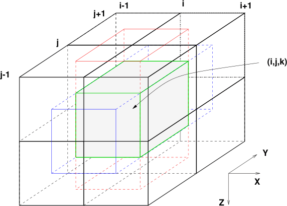
If we go from 1D to 2D conditions, we have conductivities between each four nodes. The red point is constructed by its four neighbors to the left and right, and to the top and bottom.

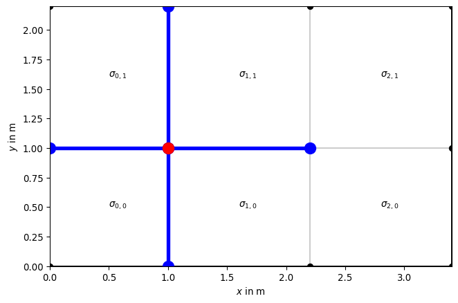
For introducing the conductivity into the coupling coefficient, there are always two values adjacent to the connecting edge.

\[ C_{i,j}^{right} = a_{i,j-1/2} / (x_{i+1}-x_{i})^2 \]

But how do we define the conductivity between the two nodes in 2D as there are two neighboring, \(a_{i,j-1}\) and \(a_{i,j}\). We need a mean, like \(a_{i,j-1/2}=(a_{i,j-1}+a_{i,j})/2\) but instead of the arithmetic, we could also use the harmonic (mean of resistivities) or geometric (logarithmic) mean. Furthermore, we can include the size of the cells as weighting functions.

\(a_{i,j-1/2}=\frac{a_{i,j-1}\Delta y_{j-1}+a_{i,j}\Delta y_{j}}{y_j+1-y_{j-1}}\)?

2.4.1 3D discretization

2.5 Parabolic PDEs - Time stepping

2.5.1 Heat transfer in 1D with periodic boundary conditions

\[ \pdv{T}{t} - a \pdv[2]{T}{z} = 0 \]

with the periodic boundary conditions:

\(T(z=0,t)=T_0 + \Delta T \sin \omega t\) (daily/yearly cycle)
\(\pdv{T}{z}(z=z_1) = 0\) (no change at depth)

and the initial condition \(T(z, t=0)=\sin \pi z\) has the analytical solution \[ T(z, t) = \Delta T e^{-\pi^2 t} \sin \pi z \]

\[ \pdv{T}{t} - \div (a\grad{T}) = \div q_s \]

\(a=\frac{k}{\rho c_p}\) [m²/s] thermal diffusivity - measure of heat transfer
\(k\) [W/m/K] thermal conductivity - measure of temperature transfer
\(c_p\) [J/kg/K] - heat capacity - measure of heat storage per mass
\(\rho\) (kg/m³) density

Water \(k\)=0.6 W/m/K, \(\rho\)=1000 kg/m³, \(c\)=4180 J/kg/K \(\Rightarrow\) \(a\)=1.43e-7 m²/s

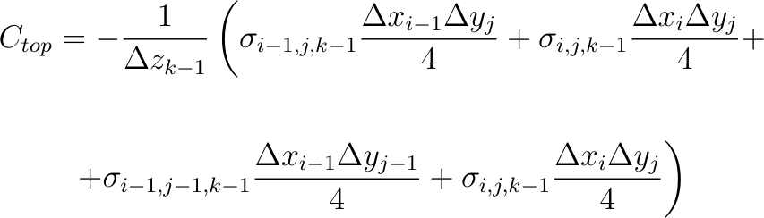
Upper boundary: daily/yearly variation

\[ T_0(t) = T_m + \Delta T \sin \omega t \]

\(T_m\) mean temperature (e.g. 12°C), \(\Delta T\) variation, e.g. 8°C

\(\omega=2\pi/t_P\) daily (\(T_d\)=3600*24s) or yearly (\(T_y=365 T_d\)) cycle ::: ::: {.column}

day = 3600 * 24
T0, dT = 12, 8
t = np.arange(100) / 50 * day
T = T0+dT*np.sin(t/day*2*np.pi)
plt.plot(t/day*24, T)
plt.xlabel("t (h)")
plt.ylabel("T (°C)")
plt.grid()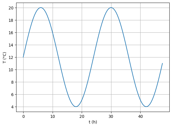

2.5.1.1 Solution by separation of variables

\[ \pdv{T}{t} = a\pdv[2]{T}{z} \]

\(T(t, z)/\Delta T - T_0 = \theta(t) Z(z)\)

\[ Z \pdv{\theta}{t} = a \theta \pdv[2]{Z}{z} \]

\[ \frac1\theta \pdv{\theta}{t} = C = a \frac{1}{Z}\pdv[2]{Z}{z} \]

regarding the BC \(e^{\imath\omega t}\) leads to \(C=\imath\omega\) and thus \(\theta=\theta_0 e^{\imath\omega t}\)

\[ \pdv[2]{Z}{z} - \imath \frac{\omega}{a} Z = \pdv[2]{Z}{z} + n^2 Z = 0 \]

Helmholtz equation with solution \(Z=Z_0 e^{\imath n z}\) (\(n^2=\imath\omega/a\))

\[ Z=Z_0 e^{\imath n z} = Z_0 e^{\sqrt{\imath\omega/a}z} = Z_0 e^{\sqrt{\omega/2a}(1+\imath)z} \]

\[ T(t, z)/\Delta T + T_0 = Z(z)\theta(t)= Z_0\theta_0 e^{-\sqrt{\omega/2a}z} e^{i(\omega t-\sqrt{\omega/2a}z)} \]

2.5.1.2 Interpretation

replacing the term \(\sqrt{2a/\omega}=\sqrt{a t_P/\pi}=d\) leads to

\[ T(z, t) = T_0 + \Delta T e^{-z/d} \sin(\omega t - z/d) \]

exponential damping of the temperature variation with decay depth \(d\)
phase lag \(z/d\) increases with depth, \(z_\pi=\sqrt{2 a/\omega}\pi=\sqrt{a t_P \pi}\)

Daily cycle: decay depth \(d\)=6cm, minimum depth=20cm
Yearly cycle: decay depth \(d\)=1.2m, minimum depth=4m

2.5.1.3 Depth profiles

a = 1.5e-7
year = day*365
d = sqrt(a*year/pi)
t = np.arange(0, 1, 0.1) * year
z = np.arange(0, 6, 0.1)
fig, ax = plt.subplots()
for ti in t:
    Tz = np.exp(-z/d)*np.sin(ti*2*pi/year-
                             z/d) * dT + T0
    ax.plot(Tz, z, label="t={:.1f}".format(
        ti/year))

ax.invert_yaxis()
ax.legend()
ax.grid()

2.5.1.4 Temporal behaviour

t = np.arange(0, 1.01, 0.01) * year
z = np.arange(0, 3, 0.4)
fig, ax = plt.subplots()
for zi in z:
    Tt = np.exp(-zi/d)*np.sin(t*2*pi/year-
                              zi/d) * dT + T0
    ax.plot(t/year*12, Tt, label=f"z={zi:.1f}")

ax.set_xlim(0, 12)
ax.set_xlabel("t (months)")
ax.set_ylabel("T (°C)")
ax.legend()
ax.grid()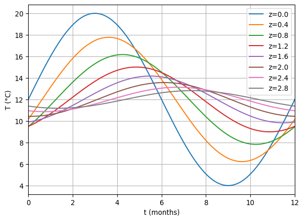

2.5.2 Explicit method

\[ \pdv{T}{t} - a \pdv[2]{T}{z} = 0 \]

Solve Poisson equation \(\div(a\grad u)=f\)

for every time step \(i\) (using FDM, FEM, FVM etc.)

Finite-difference step in time: update field by \[ T_{i+1} = T_i + a \pdv[2]{u}{z} \cdot \Delta t\]

The new field is constructed by old fields only, expressed in the difference stencil (the green line represents time stepping)

2.5.3 Implicit (Euler) method

\[ \pdv{T}{t}^n \approx \frac{T^{n+1}-T^n}{\Delta t} = a \pdv[2]{T}{z} ^{n+1} \]

Rearranging for time steps (new left and old right), this leads to

\[ T^{n+1} - \Delta t a \pdv[2]{T}{z}^{n+1} = T^n \]

Term \(a \pdv[2]{T}{z}^{n+1}\) is represented by the system matrix \(\vb A\) so that we can write

\[ \vb T^{n+1} - \vb A \vb T^{n+1} = (\vb I - \vb A) \vb T^{n+1} = \vb T^n \]

As \(\vb A\) involves the neighbors, which are only from the new time step, this is expressed in the backward stencil difference stencil

2.5.4 Mixed - Crank-Nicholson method

As the finite difference in time is centered around the mean times, it seems plausible to use the temporal mean value of \(T\)

\[ \pdv{T}{t}^n \approx \frac{T^{n+1}-T^n}{\Delta t} = \frac12 a \pdv[2]{T}{z} ^n + \frac12 a \pdv[2]{T}{z} ^{n+1} \]

Multiplying with 2 and rearranging new and old values leads to

\[ 2 T^{n+1} - \Delta t a \pdv[2]{T}{z}^{n+1} = 2 T^n + \Delta t a \pdv[2]{T}{z}^n \]

Like for the implicit method, the operator is expressed by the system matrix \(\vb A\), leading to

\[ 2\vb T^{n+1} + \vb A \vb T^{n+1} = (2\vb I + \vb A) \vb T^{n+1} = (2\vb I - \vb A) \vb T^n \]

So the new value is computed not only from its current neighbors, but also the second derivative apparent in the previous time step, expressed by the (mixed) finite difference stencil.

To summarize all three methods, the following table is created

Explicit:		\(\vb u^{n+1}\)	\(=\)	\((\vb I - \Delta t \vb A)\)	\(\vb u^n\)
Implicit:	\((\vb I + \Delta t \vb A)\)	\(\vb u^{n+1}\)	\(=\)		\(\vb u^n\)
Mixed:	\((2\vb I + \Delta t \vb A)\)	\(\vb u^{n+1}\)	\(=\)	\((2\vb I - \Delta t \vb A)\)	\(\vb u^n\)

2.6 Hyberbolic equations

Acoustic wave equation in 1D \[ \pdv[2]{u}{t} - c^2\pdv[2]{u}{x} = 0 \]

\(u\)..pressure/velocity/displacement, \(c\)..velocity

Damped (mixed parabolic-hyperbolic) wave equation \[ \pdv[2]{u}{t} - a\pdv{u}{t} - c^2\pdv[2]{u}{x} = 0 \]

2.6.1 Discretization

\[ \pdv[2]{u}{t}^{n} \approx \frac{u^{n+1}-u^n}{\Delta t} - \frac{u^{n}-u^{n-1}}{\Delta t} \]

\[ = \frac{u^{n+1}+u^{n-1}-2 u^n}{\Delta t^2} = c^2\pdv[2]{u}{x}^n \]

\[ u^{n+1} = c^2 \Delta t^2 \pdv[2]{u}{x}^{n} + 2 u^n - u^{n-1} \]

\[ \vb u^{n+1} = (\frac{1}{\Delta t}\vb A + 2\vb I) \vb u^n - \vb u^{n-1} \]

2.6.2 Example: velocity distribution

import numpy as np
import matplotlib.pyplot as plt
x=np.arange(0, 600.01, 0.5)
c = 1.0*np.ones_like(x) # velocity in m/s
c[100:300] = 1 + np.arange(0,0.5,0.0025)
c[900:1100] = 0.5  # low velocity zone

# Plot velocity distribution.
plt.plot(x,c,'k')
plt.xlabel('x [m]')
plt.ylabel('c [m/s]')
plt.grid()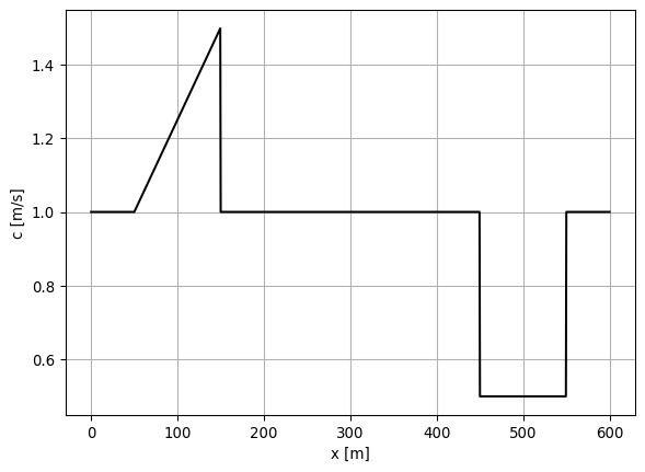

2.6.3 Initial displacement

Derivative of Gaussian (Ricker wavelet)

l=5.0

# Initial displacement field [m].
u=(x-300.0)*np.exp(-(x-300.0)**2/l**2)
# Plot initial displacement field.
plt.plot(x,u,'k')
plt.xlabel('x [m]')
plt.ylabel('u [m]')
plt.title('initial displacement field')
plt.show()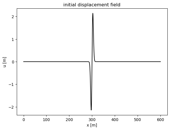

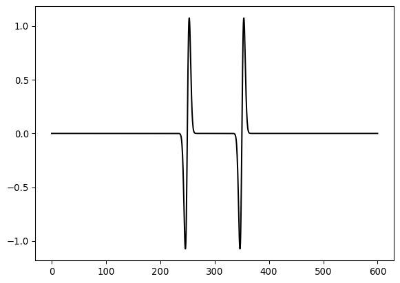
2.6.4 Time propagation

u_last=u
dt = 0.5
ddu = np.zeros_like(u)
dx = np.diff(x)
for i in range(100):
    dudx = np.diff(u)/dx
    ddu[1:-1] = np.diff(dudx)/dx[:-1]
    u_next = 2*u-u_last+ddu*c**2 * dt**2
    u_last = u
    u = u_next

plt.plot(x,u,'k')