Show the code
Ginv = np.linalg.inv(G.T @ G) @ G.T
RM = Ginv@G
RD = G@Ginv
im = plt.imshow(RD, vmin=-1, vmax=1, cmap="bwr")
plt.colorbar(im)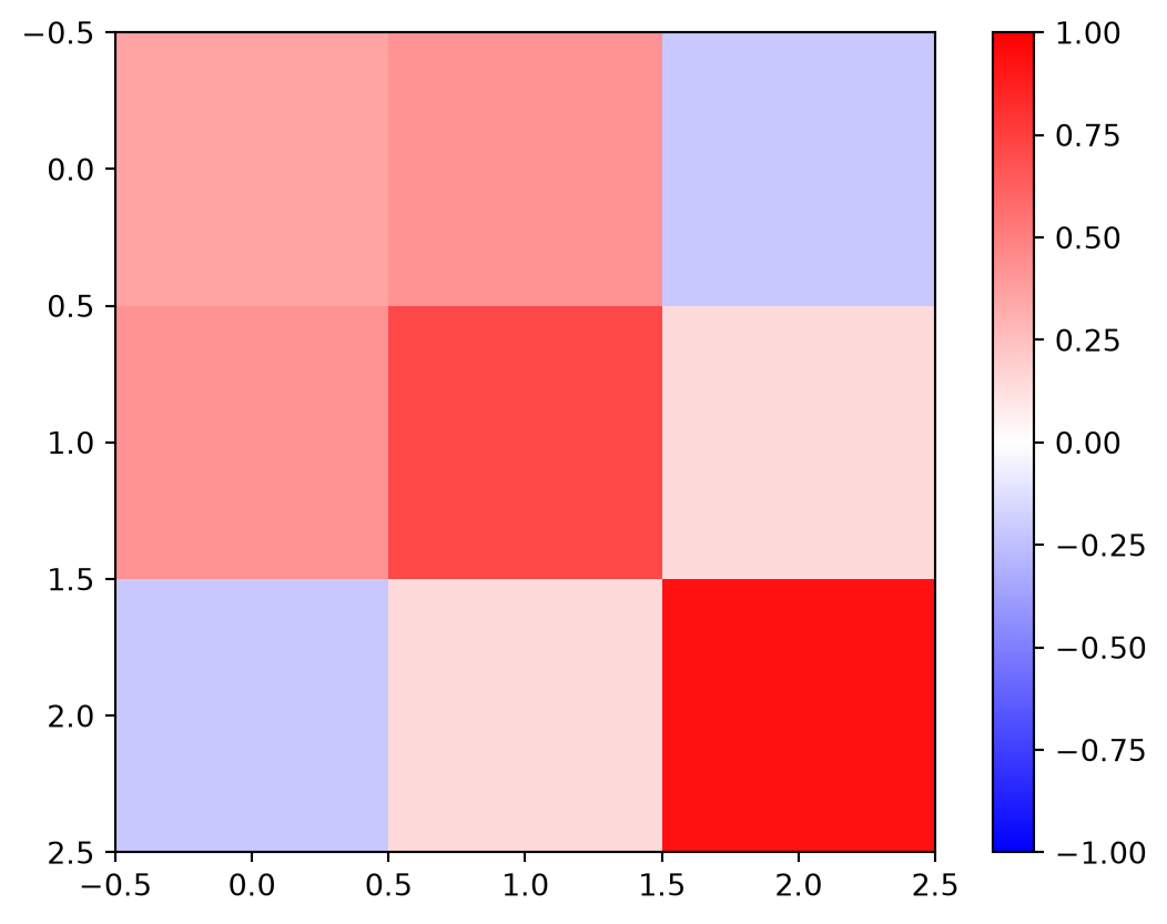
After having a solution (e.g. the least-squares solution, but generally), there are a couple of questions that can be summarized with the term resolution:
We start with the data consisting of a true model \(\vb m^\text{true}\) \[\vb d= \vb G \vb m^\text{true} + \vb n\]
If we do a matrix inversion with any inverse operator \({\vb G}^\dagger\), we obtain our model estimate \({\vb m}^\text{est}\) by application to \(\vb d\) \[{\vb m}^\text{est} = {\vb G}^\dagger {\vb d}= {\vb G}^\dagger{\vb G}{\vb m}^\text{true} + {\vb G}^\dagger{\vb n} = \]
The first term on the right-hand side is the combination of forward and inverse operator, projecting from model to data and back to model, and is therefore called model resolution matrix \({\vb R}^M={\vb G}^\dagger{\vb G}\):
\[\vb m^\text{est} = {\vb R}^M {\vb m}^\text{true} + {\vb G}^\dagger{\vb n}\]
\(\vb R^M\) obviously tells us how is the true model (\({\vb m}^\text{true}\)) is reflected in our estimate (\({\vb m}^\text{est}\)). Every column of the matrix can be interpreted as a so-called point-spread function, i.e. how a single anomaly is distributed in the model space.
The diagonal elements of \(\vb R^M\) states how well the individual points are reflected correctly and can therefore be treated as resolution of individual parameters and plotted like a model, mostly between 0 and 1. Ideally, \(\vb R^M\) is an identity matrix, but mostly it deviates from it.
Let’s put it the other way round: How well are observed data \(d^\text{obs}\) explained by our model? We again use the model
\[{\vb m}^\text{est} = {\vb G}^\dagger {\vb d}^\text{obs}\]
and project into the data space
$${d}^ = {G}{m}^ = {G}{G}^^
The first term on the right-hand side projects from data to model and back to data and is therefore called data resolution or data importance (or information density) matrix \({\vb R}^D={\vb G}{\vb G}^\dagger\), so that
\[{\vb d}^\text{est} = {\vb R}^D {\vb d}^\text{obs}\]
It tells us how the individual data are correlated with each other. The diagonal of \(R^D\) bears the information content of the individual data contributing to the model and can be plotted like any data vector .
\[{\vb G}^\dagger=({\vb G}^T{\vb G})^{-1} {\vb G}^T\]
\[\Rightarrow {\vb R}^M = ({\vb G}^T{\vb G})^{-1} {\vb G}^T {\vb G}= {\vb I}\]
perfect model resolution
\[{\vb G}^\dagger=({\vb G}^T{\vb G})^{-1} {\vb G}^T \quad \Rightarrow \quad {\vb R}^D = {\vb G}({\vb G}^T{\vb G})^{-1} {\vb G}^T\]
Ginv = np.linalg.inv(G.T @ G) @ G.T
RM = Ginv@G
RD = G@Ginv
im = plt.imshow(RD, vmin=-1, vmax=1, cmap="bwr")
plt.colorbar(im)
sum(diag(RD)) \(\Rightarrow\) 2x = np.arange(0, 3, 0.1)
x[-1] = 3.5
err = 0.1
d = 0.5-0.5*x + np.random.randn(len(x)) * err
A = np.ones((len(x), 2))
A[:, 1] = x[:]
Ainv = np.linalg.inv(A.T @ A) @ A.T
m = Ainv @ d
print("m = ", m)
fig, ax = plt.subplots()
ax.plot(x, d, "b+")
ax.plot(x, A@m, "r-")
ax.grid()
residual = A @ m - d
print("mean=", np.mean(residual))
print("std=", np.std(residual))
print("X²=", np.sqrt(np.mean((residual/err)**2)))m = [ 0.47881015 -0.46971096]
mean= 1.295260195396016e-17
std= 0.08725032651333633
X²= 0.8725032651333633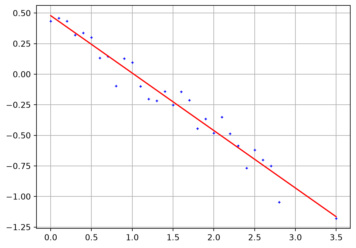
RD = A @ Ainv
fig, ax = plt.subplots(figsize=(7,6))
im = ax.matshow(RD, cmap="bwr",
    vmin=-0.3, vmax=0.3)
plt.colorbar(im);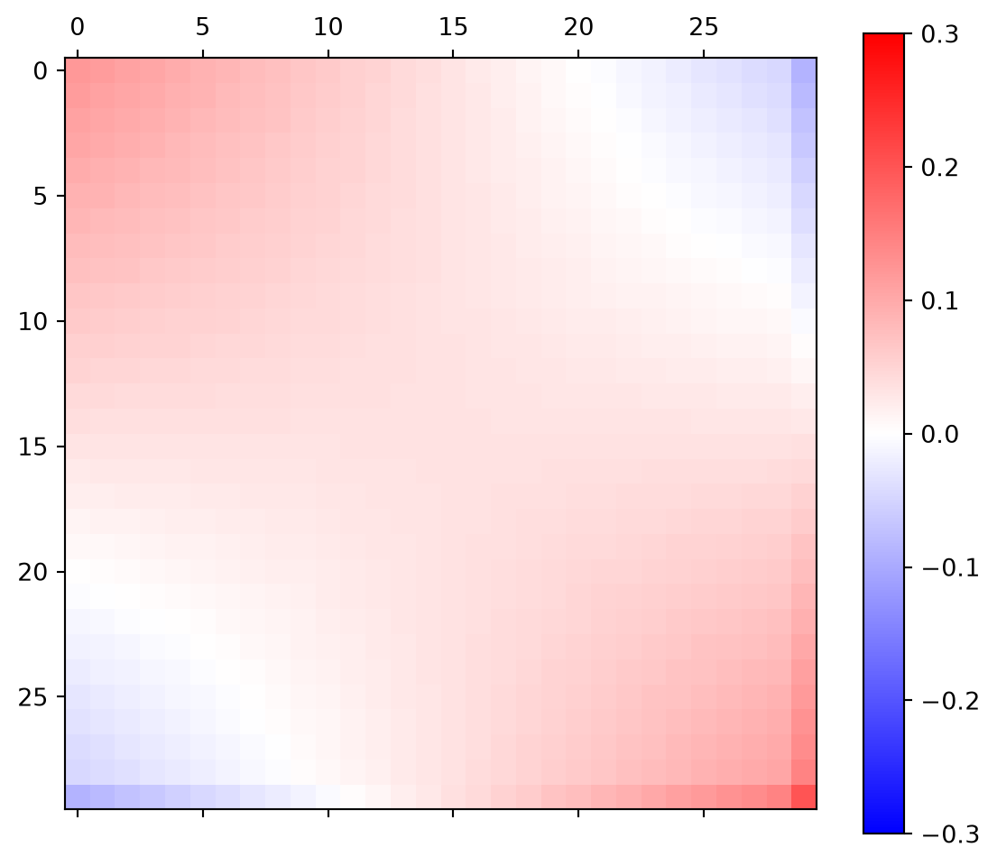
rd = np.diag(RD)
display(np.sum(rd))
plt.plot(x, rd, "+-", ms=5);
np.float64(1.9999999999999996)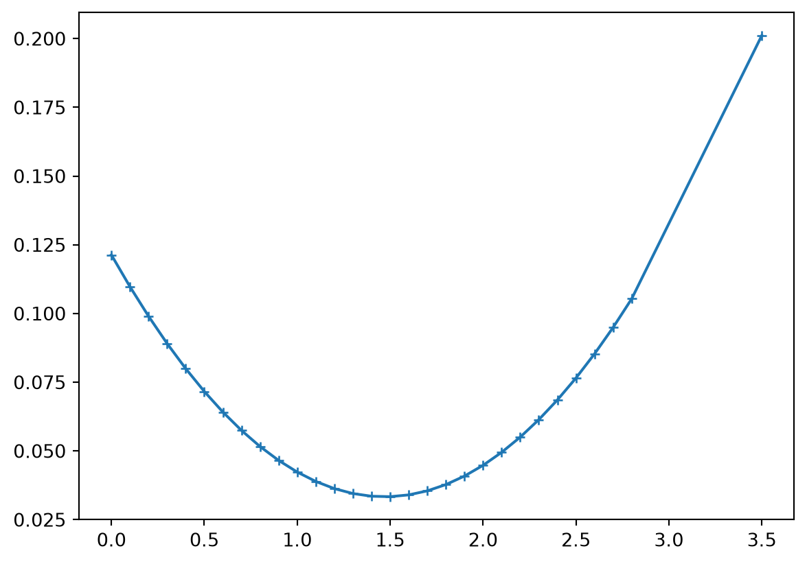
Unweighted residual norm (root-mean square RMS)
\[\|{\bf d}-{\bf f}({\bf m})\| = \sqrt{1/N\sum (d_i-f_i({\bf m}))^2}\]
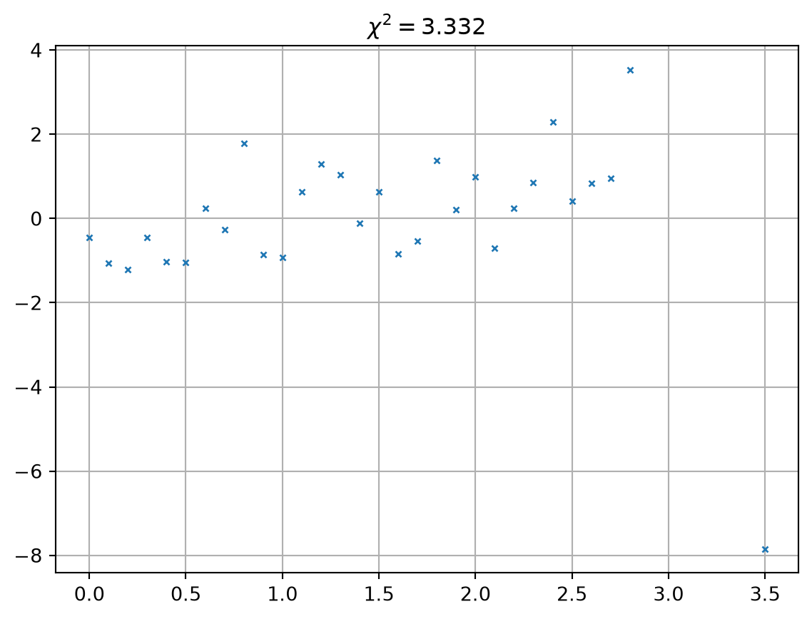
Weighting by individual error \(\epsilon_i\) (chi-square value):
\[\chi^2=\frac1N \sum \left( \frac{d_i-f_i({\bf m})}{\epsilon_i} \right)^2 \rightarrow \min\]
In case of exact error estimates: \(\chi^2=1\)
replace \(d_i\) by \(\hat{d}_i=d_i/\epsilon_i\) leads to \[{\bf m}= (\hat{\bf G}^T\hat{\bf G})^{-1} \hat{\bf G}^T \hat{\bf d}\] with \(\hat{{\bf G}}=\mbox{diag}(1/\epsilon_i)\cdot {\bf G}\)
The \(L_2\) norm is the rooted sum of squared elements of a vector \(\bf v\):
\[\Phi^P=\|{\bf v}\|_2=\sqrt{\sum_i v_i^2}\]
More generally, the \(L_P\) norm is computed by \[\Phi^P=\|{\bf v}\|_P=\left( \sum_i |v_i|^P \right)^{1/P}\]
\[\Phi^1=\|{\bf v}\|_1=\sum_i |v_i|\]
By the ratio of its contribution to L1 and L2 norm we can reweight \(\epsilon_i\) \[ w_i = \frac{|v_i|/\|\vb v\|^1_1}{v_i^2/\|\vb v\|^2_2} = \frac{\|\vb v\|^2_2}{|v_i| \cdot \|\vb v\|^1_1} \]
This is known as Iteratively Reweighted Least-Squares (IRLS)
d[-1] += 1
m = Ainv @ d
print("m = ", m)
fig, ax = plt.subplots()
ax.plot(x, d, "b+")
ax.plot(x, A@m, "r-")
ax.plot(x, 0.5-0.5*x, "m--")
ax.grid()
m = [ 0.39065588 -0.38706633]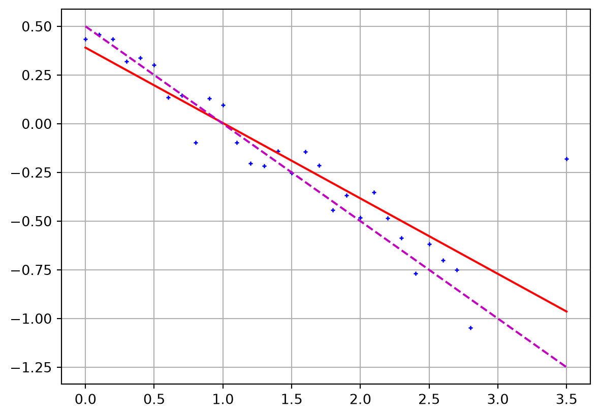
Always have a look at the misfit distribution (not only \(\chi^2\))
number of independent columns and rows, i.e. the degree of non-degenerateness.
\[ \textbf{G}=\mqty(1 & 1 & 0 \\ 0 & 0 & 1) \]
\[ \textbf{G}=\mqty(1 & 1 & 0 \\ 0 & 0 & 1) \]
adding data 1+2
\[ \textbf{G}=\mqty(1 & 1 & 0 \\ 0 & 0 & 1 \\ 1 & 1 & 1) \]
does not help, because they are linear dependent (\(rk({\bf G})=2\)).
Analog to the least-squares inverse \(({\bf G}^T {\bf G})^{-1} {\bf G}^T\) there is an inverse for under-determined problems:
\[ \bf m = G^T (G G^T)^{-1} d = G^\dagger d \]
that is called minimum-norm solution.
The backslash operator (G\d) yields the minimum-norm solution.
From the models fulfilling \(\bf G m=d\) we are looking for the “smallest”
\[ \text{min} \Phi=\bf m^T m \quad\mbox{with}\quad G m=d \]
We use the method of Lagrangian parameters (\(\lambda_i\)) \[ \Phi = \bf m^T m + \lambda^T (G m - d) \rightarrow \mbox{min} \]
The derivatives vanish
\[ \frac{\partial\Phi}{\partial \lambda} = \bf G m - d=0 \]
\[ \frac{\partial\Phi}{\partial m} = 2\bf m^T + {\bf \lambda}^T G = 0 \]
\[ \Rightarrow {\bf m} = -\frac{1}{2} ({\lambda}^T {\bf G})^T = -\frac{1}{2}{\bf G}^T \lambda \]
from which we can determine the Langrangian parameters
\[ \lambda = -2 ({\bf G G^T})^{-1} \bf d \]
Replacing them we obtain the minimum-norm solution \[ {\bf m}_{MN} = \bf G^T (G G^T)^{-1} d \]
\[ \bf G^\dagger = G^T (G G^T)^{-1} \]
\[ {\bf R}^M = \bf G^\dagger G = G^T (G G^T)^{-1} G \]
\[ {\bf R}^D = \bf G G^\dagger = G G^T (G G^T)^{-1} = I \]
For underdetermined problems, all data are independent and equally important. Model parameters are insufficiently resolved.
\[ \Rightarrow \vb R^M=\vb G^\dagger \vb G=(\vb G^T \vb G + \lambda \vb C^T \vb C)^{-1} \vb G^T \vb G \]
A column represents how a cell anomaly is “spread” (Friedel 2003).
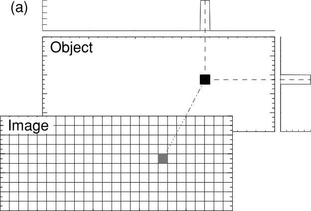
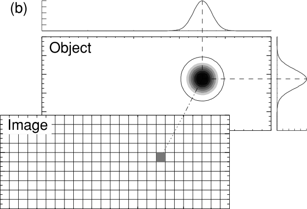
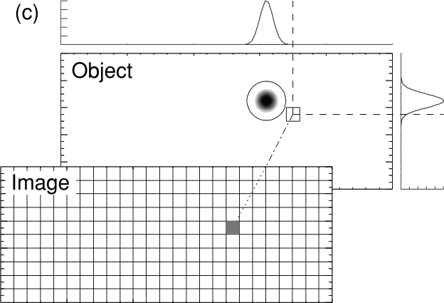
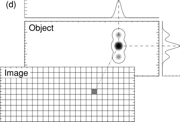
states how a single model cell can be retrieved

How big needs a sphere to be to integrate a value of 1 (perfect resolution)?
Resolution radius \[ r = \frac{r_i}{\sqrt{\vb R^M_{ii}}}=\frac{\sqrt{A_i/\pi}}{\sqrt{\vb R^M_{ii}}} \]