12 Example VES inversion

In this example, we will exemplify non-linear minimization by using vertical electrical soundings in 1D. To this end, we import two types of forward operators:

VESModelling uses a block discretization of (few) \(N\) layer resistivities preceded by N-1 thickness values
VESRhoModelling uses a fixed (many) layer discretization that is adressed by smoothness constraints

Show the code

from pygimli.physics.ves import VESModelling, VESRhoModelling
from pygimli.viewer.mpl import drawModel1D

The first is used for creating the synthetic model and to demonstrate the Levenberg-Marquardt algorithm. The second stands for all types of (also 2D and 3D) discretizations using a smoothness-constrained (Occam) inversion.

12.1 The synthetic model

The experiment comprises a VES sounding with AB/2 values between 6m and 1km. The synthetic model consist of a 20m thick bad conductor embedded in rather conductive halfspace with 10m overburden. Gaussian noise with a relative error model of 3% is added to the data.

Show the code

ab2 = np.logspace(0.5, 3, 30)
fBlock = VESModelling(ab2=ab2, mn2=ab2/3, nLayers=3)
error = 0.03
modelSynth = [10, 20, 20, 500, 30]
data = fBlock.response(modelSynth)
data *= np.random.normal(1, error, len(ab2))
print(data)

30 [20.686978036849204, 20.38349679149489, 20.510608338690187, 21.13993028920831, 20.836201776280745, 21.52013435504813, 22.67159048910943, 25.452191975187727, 30.317240592031602, 34.12411845055125, 38.66976454183282, 46.81704566659458, 54.018514020986984, 58.1754347315536, 75.04112290860583, 74.6030663175021, 83.27685330650817, 89.84863271660582, 96.21939380550589, 96.8810732152488, 85.79764752476778, 87.30338561444887, 76.70908525525306, 68.17804577147672, 54.393401041197116, 44.66861039271677, 37.030186258334126, 33.193663610678726, 33.02258474753975, 30.758836877925805]

Show the code

fig, ax = plt.subplots()
ax.loglog(data, ab2, "x")
ax.invert_yaxis()
ax.grid()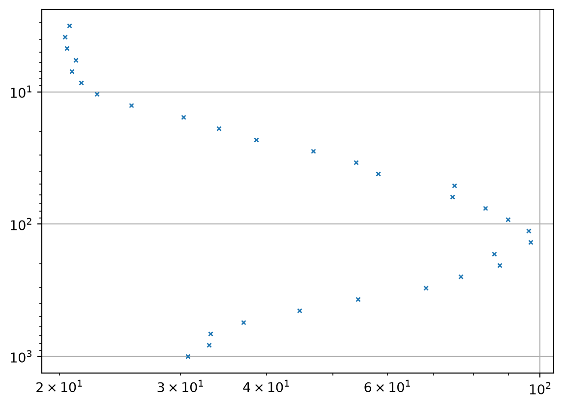

The intrinsic model parameters and data are resistivity and apparent resistivity. For both data and model we use a logarithmic transform For computing the Jacobian by a Finite Difference (brute force) approach we write a function taking this into account:

Show the code

def Jacobian(model, f):
    J = np.zeros([len(ab2), len(model)])
    responseLog = np.log(f(model))
    for i in range(len(model)):
        modelNew = model.copy()
        modelNew[i] *= 1.1
        J[:, i] = (np.log(f(modelNew))-responseLog) / (np.log(modelNew[i]) - np.log(model[i]))

    return J

In deteministic non-linear minimization approaches we start from a starting model \(m^0\) and improve the model iteratively by adding a model update \(\Delta \vb m\) so that \(\vb m^{n+1}=\vb m^n+\Delta\vb m^n\), based on the data misfit \(\Delta \vb d=\vb d-\vb f(\vb m^n)\) and the Jacobian matrix \(\vb J=\pdv{f(\vb m)}{m}\). For stopping the inversion, several criteria are used:

a maximum iteration number is reached (typically 10-20)
the objective function stagnates
the target data fit is reached (\(\chi^2=1\))

In the following, we always use error-scaled properties, i.e. \(\vb J\), \(\vb d\) and \(\vb f\) are scaled by the relative data error.

12.2 Levenberg-Marquardt algorithm

This method is typical for small parameter numbers like curve fits or block models, where the parameters are not related to each other. It uses only a local damping the least-squares solution of the linearized inverse problem \(\vb J \Delta\vb m=\Delta \vb d\).

\[\Delta\vb m = (\vb J^T \vb J + \lambda \vb I)^{-1} (\vb J^\top (\vb d-\vb f(\vb m)))\]

The damping parameter \(\lambda\) is for stabilization in the early stage and decreased subsequently.

We start the inversion with a homogeneous model and compute its Jacobian matrix:

Show the code

model = np.array([15, 15, 100, 100, 100])
J = Jacobian(model, fBlock)
plt.imshow(J.T, cmap="bwr", vmin=-1, vmax=1);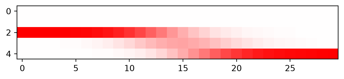

The thickness values show no sensitivity as the model is homogeneous. The three layers exhibit increased sensitivities for small, medium and large AB/2 values.

12.2.1 Inversion

The inversion is then done by solving the damped normal equations in every iteration.

Show the code

model = np.array([15, 15, 100, 100, 100])
I = np.eye(len(model))
lam = 100
for i in range(5):
    response = fBlock(model)
    J = Jacobian(model, fBlock) / error
    dData = (np.log(data) - np.log(response)) / error
    print("chi2 = ", np.mean(dData**2))
    dm = np.linalg.inv(J.T@J + I*lam) @ (J.T@dData)
    model = np.exp(np.log(model) + dm)
    lam *= 0.8

print(model)

chi2 =  1106.635417512626
chi2 =  58.802811924731195
chi2 =  1.957139509651203
chi2 =  1.3161965419993509
chi2 =  1.31583670165712
[ 10.22086153  17.54723813  20.01228196 585.03064113  29.11101175]

We plot the data fit and the model along with the synthetic model

Show the code

fig, ax = plt.subplots(ncols=2)
ax[0].loglog(data, ab2, "x", label="data")
ax[0].loglog(response, ab2, "-", label="response")
ax[0].invert_yaxis()
ax[0].legend()
ax[0].grid()
drawModel1D(ax[1], model=modelSynth, label="synthetic")
drawModel1D(ax[1], model=model, label="result")
ax[1].invert_yaxis()
ax[1].legend()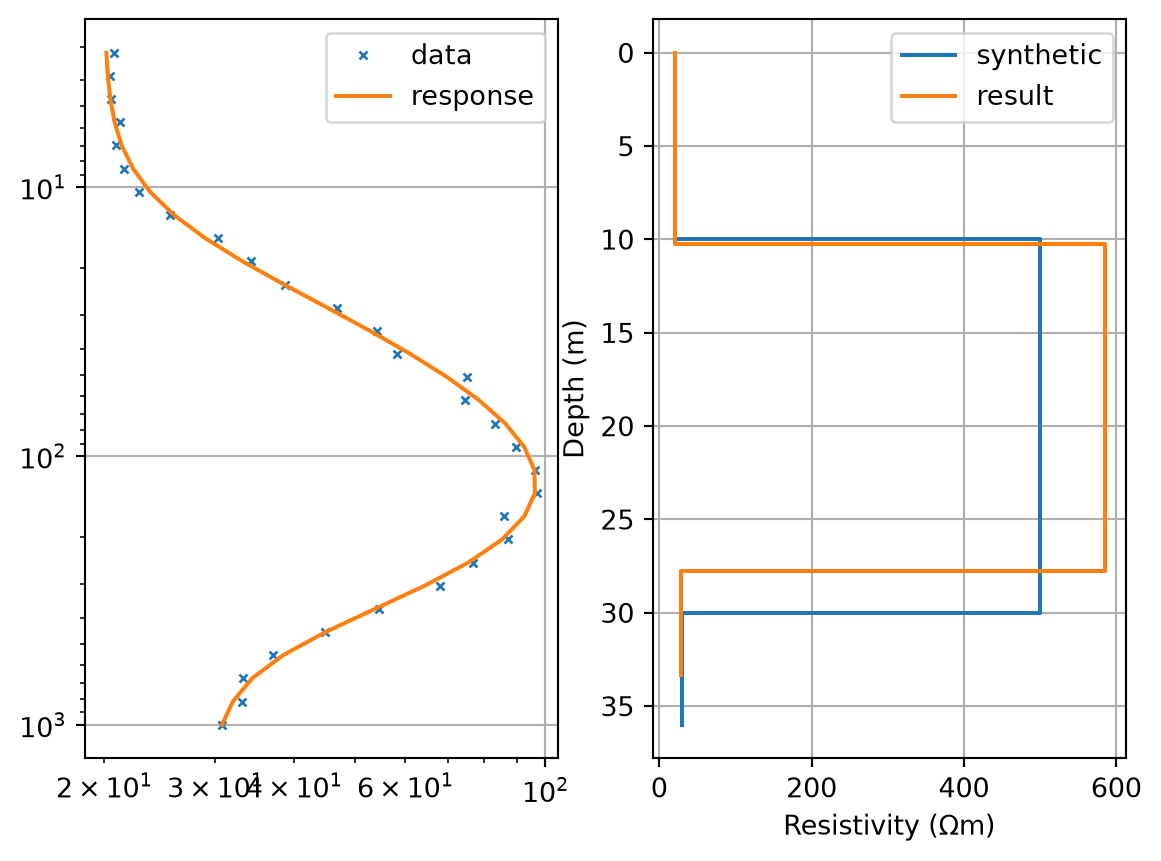

12.2.2 Resolution and model covariance

Let us start with the data resolution matrix

Show the code

JTJ = J.T@J
DRM = J@np.linalg.inv(JTJ)@J.T
plt.imshow(DRM, cmap="bwr", vmin=-1, vmax=1);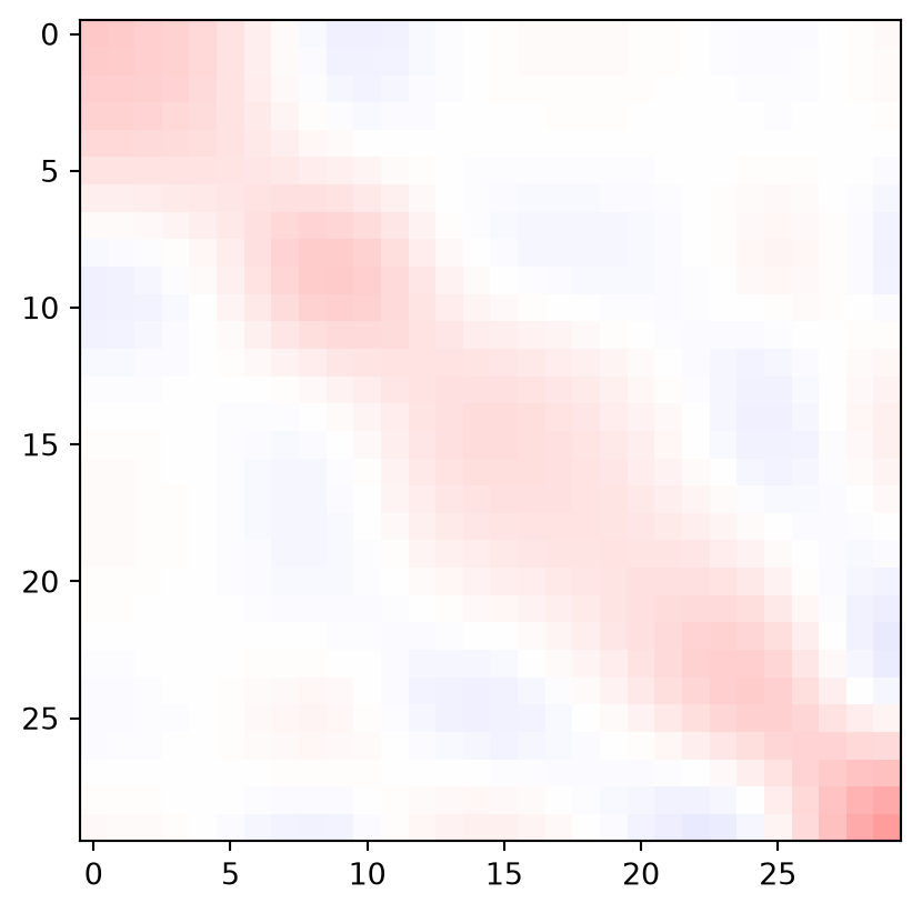

The overall information content is 5, i.e. matching the number of resolved parameters. So the individual data are weaker and neighboring AB/2 are highly correlated.

As for the overdetemined problem the model resolution is perfect, we instead compute the model covariance \[ MCM = (\vb J^T \vb J + \lambda \vb I)^{-1} \]

Show the code

MCM = np.linalg.inv(JTJ)
print(np.sqrt(np.diag(MCM)))
plt.imshow(MCM, cmap="bwr", vmin=-1, vmax=1);

[0.10127431 2.50155509 0.01433602 2.47689182 0.02232051]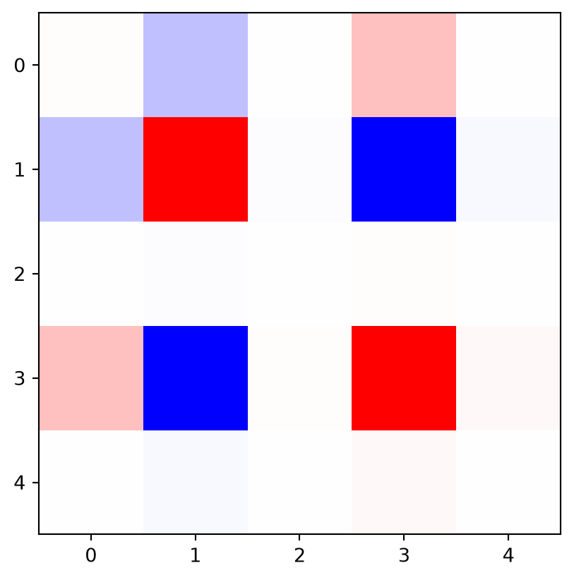

We observe a strong anti-correlation between the second layer resistivity and thickness. In total, these show higher variances than the other three parameters that are well determined (the variance is also a relative one).

12.3 Smoothness-constrained inversion

Here we use a predefined geometry (layers) with increasing layer thickness. This is passed to the forward operator in the initialization so that only the resistivity vector is passed to the forward routine. We start with a homogeneous resistivity and compute the Jacobian matrix

Show the code

thk = np.linspace(1, 10, 25)
fSmooth = VESRhoModelling(thk, ab2=ab2)
res = np.ones(len(thk)+1) * 100
J = Jacobian(res, fSmooth)
plt.imshow(J, cmap="bwr", vmin=-1, vmax=1);

15/07/26 - 13:36:50 - pyGIMLi - INFO - Found 1 regions.

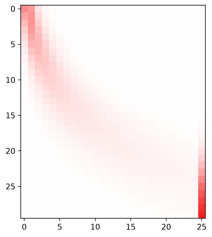
We clearly see that increasing AB/2 values (rows) shift the sensitivity towards deeper layers (columns).

12.3.1 Inversion

In the inversion, we use an explicit regularization using a roughness (gradient) operator \(\vb C\). In every iteration, we solve the regularized normal equation.

\[\Delta\vb m = (\vb J^T \vb J + \lambda \vb C^\top \vb C)^{-1} (\vb J^\top (\vb d-\vb f(\vb m)) - \lambda \vb C^\top \vb C \vb m)\]

Note the last term that arises when operating on the model itself and not only the update, i.e. the roughness of the model is taken into account.

Show the code

res = np.ones(len(thk)+1) * 100
C = np.eye(len(res)-1, len(res), 0) - np.eye(len(res)-1, len(res), k=1)
CTC = C.T@C  # only C.T C is needed
lam = 100
for i in range(6):
    response = fSmooth(res)
    J = Jacobian(res, fSmooth) / error
    dData = (np.log(data) - np.log(response)) / error
    print("chi2 = ", np.mean(dData**2))
    dm = np.linalg.inv(J.T@J + CTC*lam) @ (J.T@dData - CTC@np.log(res))
    res = np.exp(np.log(res) + dm)

chi2 =  1106.6354175126257
chi2 =  16.773504720795227
chi2 =  2.9549933376315503
chi2 =  1.3987277558308926
chi2 =  1.2182786532544772
chi2 =  1.1589954810460468

We use the function drawModel1D to plot the result along with the synthetic model. Note the two modes: a) specifying thickness and values, or b) a complete model vector with both included.

Show the code

fig, ax = plt.subplots()
drawModel1D(ax, thk, res, plot="semilogy")
drawModel1D(ax, model=modelSynth)
ax.invert_yaxis()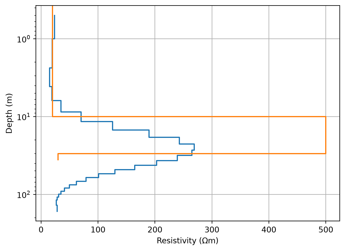

We see that the upper boundary is resolved well, but the lower boundary is smeared, a typical problem in smoothness-constrained inversion. The maximum is within the synthetic layer, but its center point moves to larger depths (where the resolution decreases). Below the smeared good conductor there is a decrease beyond the synthetic value of 30 Ohmm, before the correct value is reached for the last layer. These compensation artifacts are also known to appear.

As above, we compute the model covariance:

Show the code

JTJ = J.T@J
MCM = np.linalg.inv(JTJ + CTC*lam)
plt.imshow(MCM, cmap="bwr", vmin=-.01, vmax=.01)
var = np.sqrt(np.diag(MCM))
print(var)

[0.05733918 0.04019894 0.05047145 0.05484166 0.06683396 0.08122538
 0.09193584 0.09735016 0.0981668  0.09619235 0.09368139 0.09267707
 0.09436002 0.09876353 0.1050786  0.11222271 0.11923066 0.12537353
 0.1301187  0.13302789 0.1336267  0.13123584 0.12470726 0.11186198
 0.08759044 0.022049  ]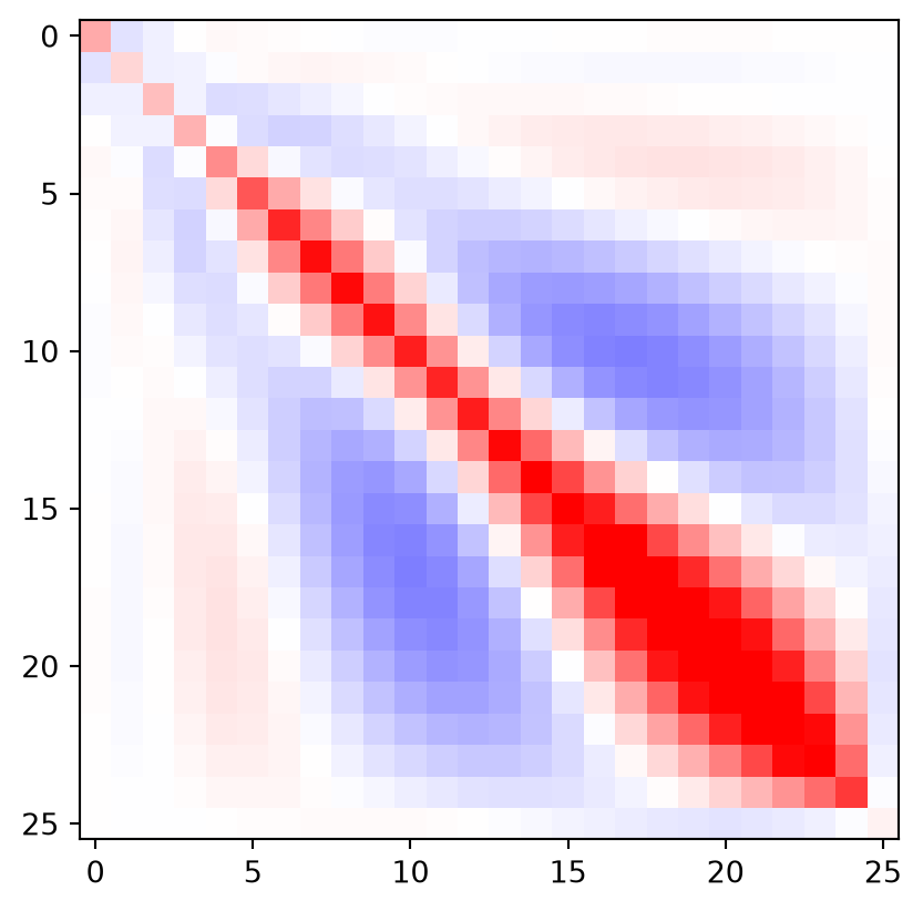

We have variances (of the logarithm, i.e. relative accuracies) in the order of 10% and can use them to plot some upper and lower resistivity bounds.

Show the code

fig, ax = plt.subplots()
drawModel1D(ax, thk, res, plot="semilogy")
drawModel1D(ax, thk, res*(1+var), color="C0", ls="--")
drawModel1D(ax, thk, res*(1-var), color="C0", ls="--")
drawModel1D(ax, model=modelSynth)
ax.invert_yaxis()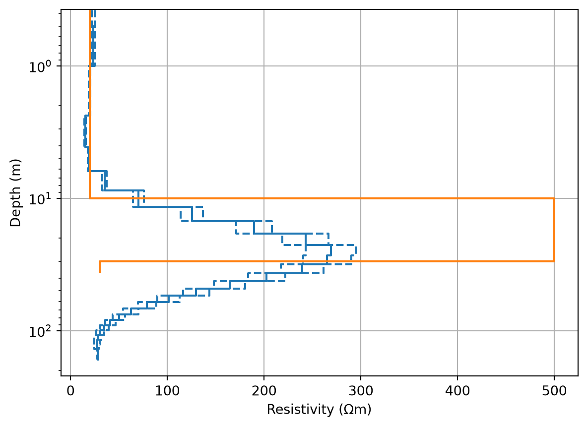

We can also compute the model resolution matrix

Show the code

MRM = np.linalg.inv(JTJ + CTC*lam) @ (JTJ)
plt.imshow(MRM, cmap="bwr", vmin=-1, vmax=1)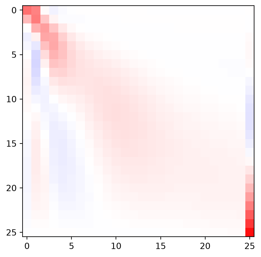

showing how much the model parameters correlate with each other. Note that even though JTJ and CTC are symmetric, the model resolution matrix is not necessarily symmetric. Every column shows how a single anomaly in the real world is projected into our model estimate, whereas every row tells where the information in one cell can come from. This is most visible for the last layer which is itself well resolved, but projects into the weakly resolved layers above. For a better balance of the model parameters, the layer thicknesses should probably be more increased with depth.