9  A simple model

Let us consider the forward response(after Menke 2012) \[f(m)= \sin(\omega m_1 x_i) + m_1 m_2\] a nonlinear function in both model parameters \(m_1\) and \(m_2\).

x = np.arange(0, 1.001, 0.05)
omega = 10
forward = lambda m: np.sin(omega * x * m[0]) + m[0] * m[1]
mSynth = [1.25, 1.25]
data = forward(mSynth);
data += np.random.randn(len(data))*0.1

We create a function for showing the objective function for a range of values

def showPhi(Phi, mrange, clim=None, ax=None):
    if ax is None:
        fig, ax = plt.subplots(figsize=(5, 5))
    if clim is None:
        clim = [np.min(Phi), np.percentile(Phi, 95)]
    ext = [mrange[0], mrange[-1], mrange[-1], mrange[0]]
    im = ax.matshow(Phi.T, extent=ext, vmin=clim[0], vmax=clim[1], cmap="Spectral_r")
    ax.set_xlabel("m1")
    ax.set_ylabel("m2")
    ax.invert_yaxis()
    # fig.colorbar(im);
    return ax

We choose a range for values of the two and compute the data objective function

mrange = np.arange(0, 2.001, 0.01)
PhiD = np.zeros([len(mrange), len(mrange)])
for i, m1 in enumerate(mrange):
    for j, m2 in enumerate(mrange):
        PhiD[i, j] = sum((data-forward([m1, m2]))**2) # + 1 * (m1-m2)**2
showPhi(PhiD, mrange)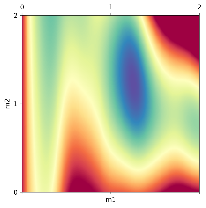

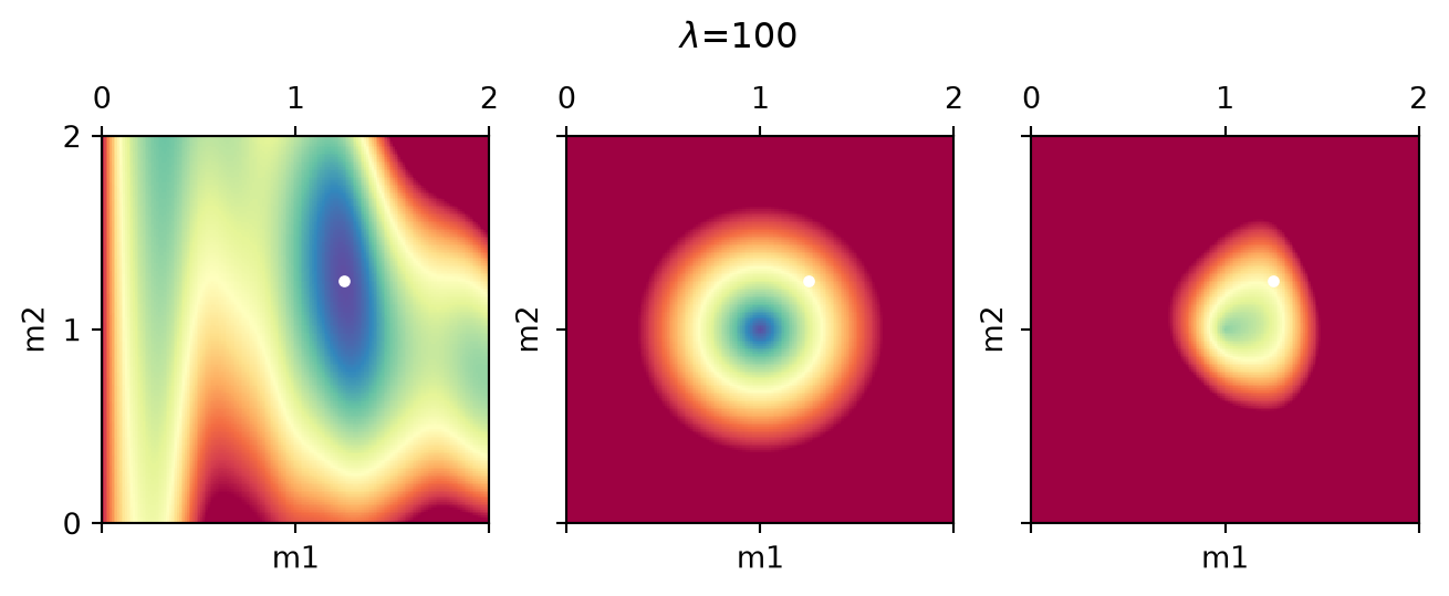
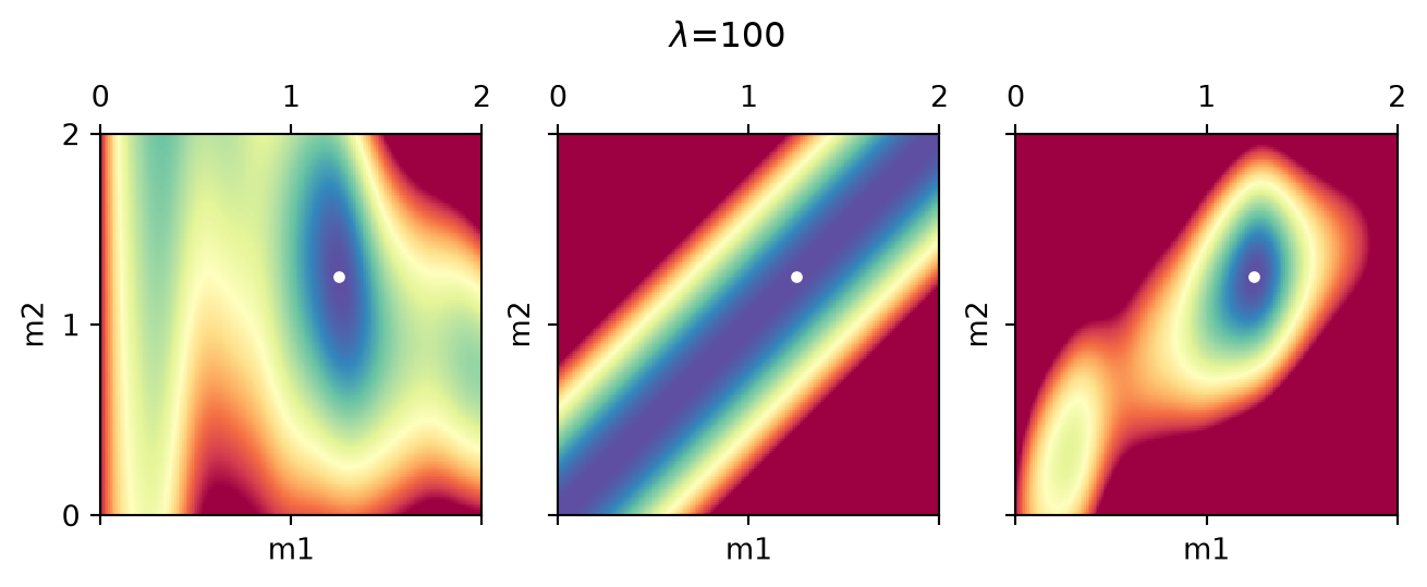
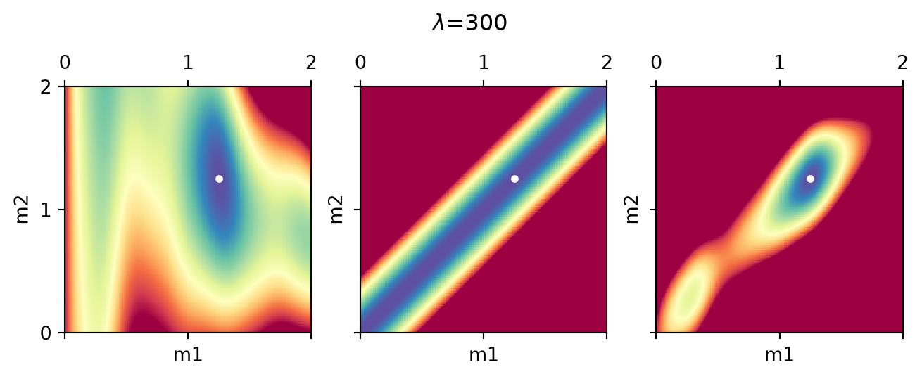
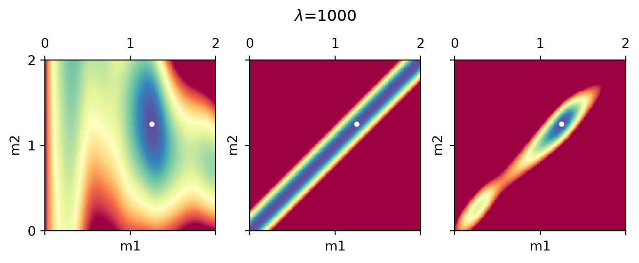
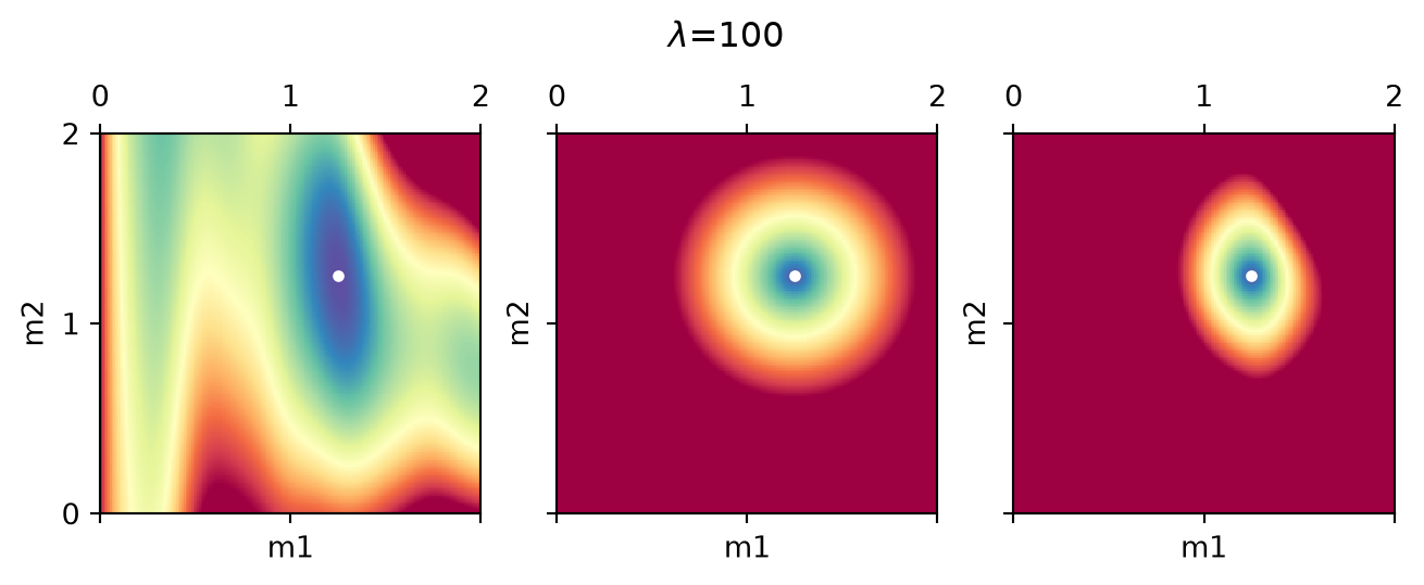
9.1 Regularization effect

\[\Phi = \Phi_d + \lambda\Phi_m\]

\(\Phi_m\): difference from reference model or smoothness

How does this regularization affect convergence?

\(\Rightarrow\) impact of regularization terms on objective function

We create another function that can show several objective functions with the same scaling

def showNPhi(Phis, mrange, clim=None):
    fig, ax = plt.subplots(ncols=len(Phis), sharex=True, sharey=True, figsize=(8, 3))
    if clim is None:
        clim = [np.min(Phis[0]), np.percentile(Phis[0], 95)]
    ext = [mrange[0], mrange[-1], mrange[-1], mrange[0]]
    for i, Phi in enumerate(Phis):
        showPhi(Phi, mrange, clim=clim, ax=ax[i])

    return ax

9.2 Smoothness

M1, M2 = np.meshgrid(mrange, mrange)
PhiM = (M1-M2)**2

for lam in [30, 100, 300, 1000]:
    ax = showNPhi([PhiD, lam*PhiM, PhiD+lam*PhiM], mrange)
    for a in ax: a.plot(1.25, 1.25, "wo")
    ax[0].figure.suptitle(rf"$\lambda$={lam}")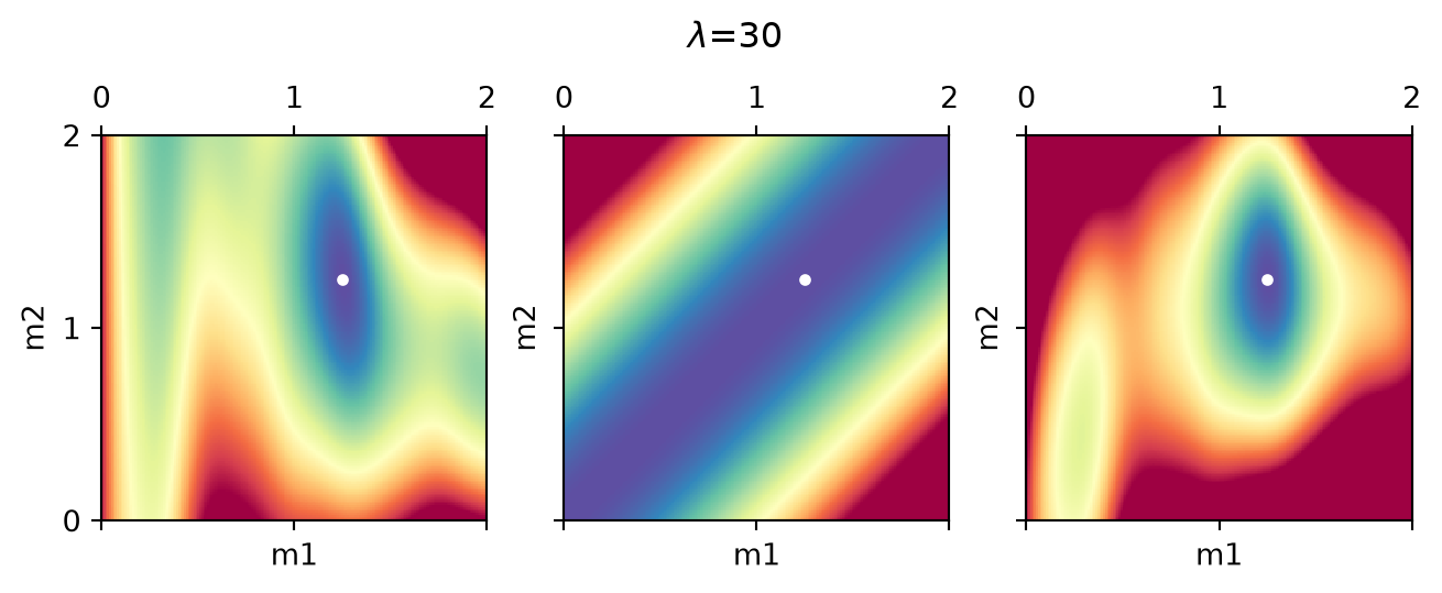

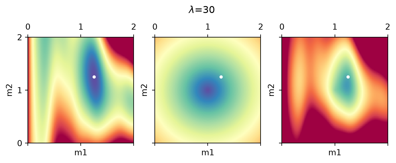
9.3 A-priori information

PhiM = np.sqrt((M1-1.25)**2+(M2-1.25)**2)
for lam in [30, 100]:
    ax = showNPhi([PhiD, lam*PhiM, PhiD+lam*PhiM], mrange)
    for a in ax: a.plot(1.25, 1.25, "wo")
    ax[0].figure.suptitle(rf"$\lambda$={lam}")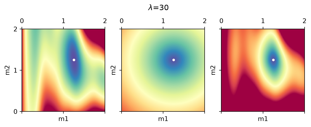

We now choose a wrong reference model

PhiM = np.sqrt((M1-1)**2+(M2-1)**2)
for lam in [100, 30]:
    ax = showNPhi([PhiD, lam*PhiM, PhiD+lam*PhiM], mrange)
    for a in ax: a.plot(1.25, 1.25, "wo")
    ax[0].figure.suptitle(rf"$\lambda$={lam}")

Menke W. 2012. Geophysical data analysis: Discrete inverse theory (Elsevier)