6  Traveltime tomography

6.1 Crosshole tomography

For this example, we use the traveltime module from pyGIMLi

import pygimli.physics.traveltime as tt

data = tt.createCrossholeData(x=[0, 10], z=-np.arange(10)-0.5)

We create a grid of

x = np.arange(10.1)  # 0 1 .. 10
y = -np.arange(0, 12.1)  # 0 1 .. 11
grid = pg.createGrid(x, y)
print(grid)
pg.show(grid);

Mesh: Nodes: 143 Cells: 120 Boundaries: 262

ax, cb = grid.show(grid.cellMarkers(), showMesh=1,
                   colorBar=False, cMap="Spectral")
sx = pg.x(data)
sy = pg.y(data)
sC = data.sensorCount()
ax.plot(sx[:sC//2], sy[:sC//2], "b*", ms=8)
ax.plot(sx[sC//2:], sy[sC//2:], "gs", ms=8)
# ax.figure.savefig("crosshole-setup.svg")
for s, g in zip(data["s"], data["g"]):
    ax.plot([sx[s], sx[g]], [sy[s], sy[g]],
            color="0.8", alpha=0.5, lw=1)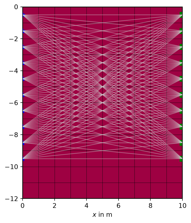

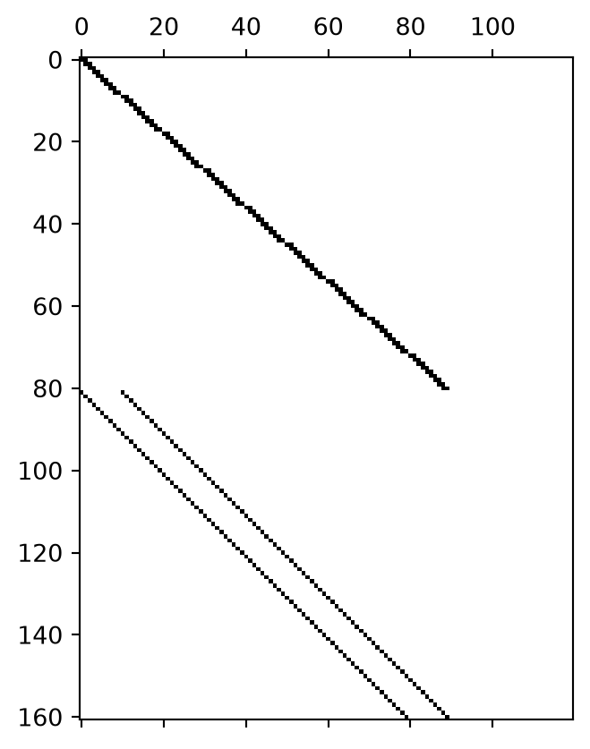
6.2 Smoothness constraints

plt.spy(C)